A unified model that covers multiple time-series tasksContinue reading on Towards Data Science »

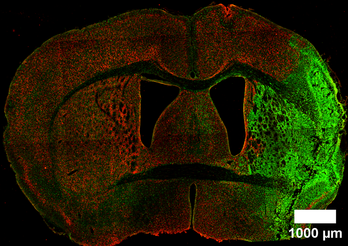
An approach using hurdle and zero-inflated models with brmsNeuN and GFAP staining in a mouse brain following cerebral ischemia. Manrique-Castano et al. (2024) (CC-BY).Counting is a fundamental task in biomedical research, particularly when analyzing cell populations. Imagine staring at countless cells within a tiny brain region — sometimes numbering in the hundreds or thousands. Yet, in other areas, these numbers may dwindle to few or even none.The challenge arises in how we analyze these counts. For large numbers, linear models, which assume a normal distribution, often serve as a reasonable approximation. Though not optimal, they provide a logical framework for initial analysis. However, the scenario shifts dramatically when cell counts are low or predominantly zeros. Here, traditional linear models (like those t-tests we run in GraphPad) falter, losing their effectiveness and relevance.As researchers, we must strive for better, going beyond t-tests and ANOVAs. This post aims to explore alternative statistical methods that more accurately reflect the realities of our data, especially when dealing with low or zero counts. By embracing more fitted approaches, we can enhance the precision of our findings and deepen our understanding of our cell populations.First, let's load the necessary libraries and create a visual theme for our plots.library(ggplot2)library(brms)library(ggdist)library(easystats)library(dplyr)library(modelr)library(patchwork)library(tibble)library(tidybayes)logit2prob <- function(logit){ odds <- exp(logit) prob <- odds / (1 + odds) return(prob)}Plot_theme <- theme_classic() + theme( plot.title = element_text(size=18, hjust = 0.5, face="bold"), plot.subtitle = element_text(size = 10, color = "black"), plot.caption = element_text(size = 12, color = "black"), axis.line = element_line(colour = "black", size = 1.5, linetype = "solid"), axis.ticks.length=unit(7,"pt"), axis.title.x = element_text(colour = "black", size = 16), axis.text.x = element_text(colour = "black", size = 16, angle = 0, hjust = 0.5), axis.ticks.x = element_line(colour = "black", size = 1), axis.title.y = element_text(colour = "black", size = 16), axis.text.y = element_text(colour = "black", size = 16), axis.ticks.y = element_line(colour = "black", size = 1), legend.position="right", legend.direction="vertical", legend.title = element_text(colour="black", face="bold", size=12), legend.text = element_text(colour="black", size=10), plot.margin = margin(t = 10, # Top margin r = 2, # Right margin b = 10, # Bottom margin l = 10) # Left margin ) What is the issue with counting zeros?In many studies, like the one shown in the graph by (1), we encounter the challenge of low cell counts, particularly where one group — marked here in black — appears to be dominated by zero counts. This scenario is not uncommon in biomedical literature, where straightforward linear models are frequently applied to analyze such data.Figure 1: CD3+ cells by Baraibar et. al (2020) (CC-BY)However, the use of these models in cases of low or zero counts can be problematic. Without access to the original datasets — which researchers often do not share — it's difficult to evaluate the efficacy of the analysis fully. To better understand this issue, let's consider a separate dataset from my own research. Several years ago, I undertook the task of counting BrdU+ cells following an ischemic event in a specific brain area called the subventricular zone (SVZ). This particular experience inclined me to evaluate more suitable statistical approaches.These are the data:Svz_data <- read.csv("Data/CellCounts.csv")Svz_data$Hemisphere <- factor(Svz_data$Hemisphere, levels = c("Contralateral", "Ipsilateral"))head(Svz_data)We can visualize that the contralateral hemisphere has a lot of null cell counts. We can have a better angle if we use a boxplot:ggplot(Svz_data, aes(x = Hemisphere, y = Cells)) + geom_boxplot() + labs(x = "Hemisphere", y = "Number of cells", title = "Cells by hemisphere") + Plot_theme + theme(legend.position = "top", legend.direction = "horizontal")Figure 2: Cell counts by hemisphereFigure 2 vividly illustrates the substantial disparities in cell counts across hemispheres. To examine what happens when we apply a typical (and horrific) linear model to such data, we'll proceed with a practical demonstration using the brms. This will help us understand the effects of these variations when analyzed under a traditional framework predicated on normal distribution assumptions.In this example, I'll fit a linear model where the factor variable “hemisphere” is the sole predictor of the cell counts:lm_Fit <- brm(Cells ~ Hemisphere, data = Svz_data, # seed for reproducibility purposes seed = 8807, control = list(adapt_delta = 0.99), # this is to save the model in my laptop file = "Models/2024-04-19_CountsZeroInflated/lm_Fit.rds", file_refit = "never")# Add loo for model comparisonlm_Fit <- add_criterion(lm_Fit, c("loo", "waic", "bayes_R2"))Are you willing to bet on what the results will be? Let's find out:If you like, you can fit a frequentist (OLS) model with lm and you will certainly get the same results. In these results, the intercept represents an estimate of cell counts for the contralateral hemisphere, which serves as our reference group. However, a significant inconsistency arises when employing a normal distribution for data that includes numerous zero counts or values close to zero. In such cases, the model is inappropriately “forced” to predict that cell counts in our hemisphere could be negative, such as -1 to -2 cells, with a confidence interval ranging from -1.5 to 3.7. This prediction is fundamentally flawed because it disregards the intrinsic nature of cells as entities that can only assume non-negative integer values.This issue stems from the fact that our model, in its current form, does not comprehend the true characteristics of the data it's handling. Instead, it merely follows our directives — albeit incorrectly — to fit the data to a linear model. This common oversight often leads researchers to further exacerbate the problem by applying t-tests and ANOVAs, thereby superimposing additional analysis onto a model that is fundamentally unsound. It is imperative that we, as researchers, recognize and harness our capabilities and tools to develop and utilize more appropriate and logically sound modeling methods that respect the inherent properties of our data.Let's plot the results using the great TidyBayes package (2) by the great Matthew KaySvz_data %>% data_grid(Hemisphere) %>% add_epred_draws(lm_Fit) %>% ggplot(aes(x = .epred, y = Hemisphere)) + labs(x = "Number of cells") + stat_halfeye() + geom_vline(xintercept = 0) + Plot_themeFigure 3: Posterior distribution for cell counts by hemisphereWe can also see this inconsistency if we perform pp_check to compare the observations with the model predictions:Figure 4: Posterior predictive checks gaussian modelOnce again, we encounter irrational predictions of cell counts falling below zero. As scientists, it's crucial to reflect on the suitability of our models in relation to the data they are intended to explain. This consideration guides us toward generative models, which are build under the premise that they could plausibly have generated the observed data. Clearly, the linear model currently in use falls short of this criterion. It predicts impossible negative values for cell counts. Let's try to find out a better model.Working with lots of zerosA zero-inflated model effectively captures the nuances of datasets characterized by a preponderance of zeros. It operates by distinguishing between two distinct processes: 1) Determining whether the result is zero, and 2) predicting the values for non-zero results. This dual approach is particularly apt for asking questions like, “Are there any cells present, and if so, how many?”For handling datasets with an abundance of zeros, we employ models such as hurdle_poisson() and Zero_inflated_poisson, both designed for scenarios where standard count models like the Poisson or negative binomial models prove inadequate (3).Loosely speaking, a key difference between hurdle_poisson() and Zero_inflated_poisson is that the latter incorporates an additional probability component specifically for zeros, enhancing their ability to handle datasets where zeros are not merely common but significant. We'll see the impact these features have in our modeling strategy using brms.Fitting a hurdle_poisson modelLet's start by using the hurdle_poisson() distribution in our modeling scheme:Hurdle_Fit1 <- brm(Cells ~ Hemisphere, data = Svz_data, family = hurdle_poisson(), # seed for reproducibility purposes seed = 8807, control = list(adapt_delta = 0.99), # this is to save the model in my laptop file = "Models/2024-04-19_CountsZeroInflated/Hurdle_Fit1.rds", file_refit = "never")# Add loo for model comparisonHurdle_Fit1 <- add_criterion(Hurdle_Fit1, c("loo", "waic", "bayes_R2"))Let's see the results using the standard summary function.summary(Hurdle_Fit1)Given this family distribution, the estimates are shown in the log scale (mu = log). In practical terms, this means that the number of cells in the contralateral subventricular zone (SVZ) can be expressed as exp(1.11) = 3.03. Similarly, the ipsilateral hemisphere is estimated to have exp(1.07) = 2.91 times the number of cells. These results align well with our expectations and offer a coherent interpretation of the cell distribution between the two hemispheres.Additionally, the hu parameter within the “Family Specific Parameters” sheds light on the likelihood of observing zero cell counts. It indicates a 38% probability of zero occurrences. This probability highlights the need for a zero-inflated model approach and justifies its use in our analysis.To better visualize the implications of these findings, we can leverage the conditional_effects function. This tool in the brms package allows us to plot the estimated effects of different predictors on the response variable, providing a clear graphical representation of how the predictors influence the expected cell counts.Hurdle_CE <- conditional_effects(Hurdle_Fit1)Hurdle_CE <- plot(Hurdle_CE, plot = FALSE)[[1]]Hurdle_Com <- Hurdle_CE + Plot_theme + theme(legend.position = "bottom", legend.direction = "horizontal")Hurdle_CE_hu <- conditional_effects(Hurdle_Fit1, dpar = "hu")Hurdle_CE_hu <- plot(Hurdle_CE_hu, plot = FALSE)[[1]]Hurdle_hu <- Hurdle_CE_hu + Plot_theme + theme(legend.position = "bottom", legend.direction = "horizontal")Hurdle_Com | Hurdle_huFigure 5: Conditional effects for the hurdle fitThese plots draw a more logical picture than our first model. The graph on the left shows the two parts of the model (“mu” and “hu”). Also, if this model is suitable, we should see more aligned predictions when using pp_check:pp_check(Hurdle_Fit1, ndraws = 100) + labs(title = "Hurdle regression") + theme_classic()Figure 6: Posterior predictive checks hurdle modelAs expected, our model predictions have a lower boundary at 0.Modeling the dispersion of the dataObserving the data presented in the right graph of Figure 5 reveals a discrepancy between our empirical findings and our theoretical understanding of the subject. Based on established knowledge, we expect a higher probability of non-zero cell counts in the subventricular zone (SVZ) of the ipsilateral hemisphere, especially following an injury. This is because the ipsilateral SVZ typically becomes a hub of cellular activity, with significant cell proliferation post-injury. Our data, indicating prevalent non-zero counts in this region, supports this biological expectation.However, the current model predictions do not fully align with these insights. This divergence underscores the importance of incorporating scientific understanding into our statistical modeling. Relying solely on standard tests without contextual adaptation can lead to misleading conclusions.To address this, we can refine our model by specifically adjusting the hu parameter, which represents the probability of zero occurrences. This allows us to more accurately reflect the expected biological activity in the ipsilateral hemisphere's SVZ. We build then a second hurdle model:Hurdle_Mdl2 <- bf(Cells ~ Hemisphere, hu ~ Hemisphere) Hurdle_Fit2 <- brm( formula = Hurdle_Mdl2, data = Svz_data, family = hurdle_poisson(), # seed for reproducibility purposes seed = 8807, control = list(adapt_delta = 0.99), # this is to save the model in my laptop file = "Models/2024-04-19_CountsZeroInflated/Hurdle_Fit2.rds", file_refit = "never")# Add loo for model comparisonHurdle_Fit2 <- add_criterion(Hurdle_Fit2, c("loo", "waic", "bayes_R2"))Let's see first if the results graph aligns with our hypothesis:Hurdle_CE <- conditional_effects(Hurdle_Fit2)Hurdle_CE <- plot(Hurdle_CE, plot = FALSE)[[1]]Hurdle_Com <- Hurdle_CE + Plot_theme + theme(legend.position = "bottom", legend.direction = "horizontal")Hurdle_CE_hu <- conditional_effects(Hurdle_Fit2, dpar = "hu")Hurdle_CE_hu <- plot(Hurdle_CE_hu, plot = FALSE)[[1]]Hurdle_hu <- Hurdle_CE_hu + Plot_theme + theme(legend.position = "bottom", legend.direction = "horizontal")Hurdle_Com | Hurdle_huFigure 7: Conditional effects for the hurdle fit 2This revised modeling approach seems to be a substantial improvement. By specifically accounting for the higher probability of zero counts (~75%) in the contralateral hemisphere, the model now aligns more closely with both the observed data and our scientific knowledge. This adjustment not only reflects the expected lower cell activity in this region but also enhances the precision of our estimates. With these changes, the model now offers a more nuanced interpretation of cellular dynamics post-injury. Let's see the summary and the TRANSFORMATION FOR THE hu parameters (do not look at the others) to visualize them in a probability scale using the logit2prob function we created at the beginning.logit2prob(fixef(Hurdle_Fit2))Although the estimates for the number of cells are similar, the hu parameters (in the logit scale) tells us that the probability for seeing zeros in the contralateral hemisphere is:Conversely:Depicts a drastic reduction to about 0.23% probability of observing zero cell counts in the injured (ipsilateral) hemisphere. This is a remarkable change in our estimates.Now, let's explore if a zero_inflated_poisson() distribution family changes these insights.Fitting a zero-inflated Poisson modelAs we modeled the broad variations in cell counts between the ipsilateral and contralateral hemispheres using the hu parameter, we'll fit as well these two parts of the model in our zero_inflated_poisson(). Here, the count part of the model uses a “log” link, and the excess of zeros is modeled with a “logit” link. These are linked functions associated to the distribution family that we'll not discuss here.Inflated_mdl1 <- bf(Cells ~ Hemisphere, zi ~ Hemisphere)Inflated_Fit1 <- brm( formula = Inflated_mdl1, data = Svz_data, family = zero_inflated_poisson(), # seed for reproducibility purposes seed = 8807, control = list(adapt_delta = 0.99), # this is to save the model in my laptop file = "Models/2024-04-19_CountsZeroInflated/Inflated_Fit.rds", file_refit = "never")# Add loo for model comparisonInflated_Fit1 <- add_criterion(Inflated_Fit1, c("loo", "waic", "bayes_R2"))Before we look at the results, let's do some basic diagnostics to compare the observations and the model predictions.set.seed(8807)pp_check(Inflated_Fit1, ndraws = 100) + labs(title = "Zero-inflated regression") + theme_classic()Figure 8: Model diagnostics for the zero-inflated regressionFrom Figure 8, we can see that the predictions deviate from the observed data in a similar way to the hurdle model. So, we have no major changes up to this point.Let's see the numerical results:logit2prob(fixef(Inflated_Fit1))Here, we do see tiny changes in the estimates. The estimate for the number of cells is similar with small changes in the credible intervals. Otherwise, the parameter for the number of zeros seems to experience a larger shift. Let's see if this has any effect on our conclusions:Indicates that there is approximately a 77% probability of observing zero counts in the reference hemisphere. Now, for the injured hemisphere, we have:Again, this signals a drastic reduction in observing zero cell counts in the injured (ipsilateral) hemisphere. Evaluating the results using scientific knowledge, I would say that both models provide similarly sound predictions. The graphical results for our zero_inflated_poisson model are as follows:Inflated_CE <- conditional_effects(Inflated_Fit1)Inflated_CE <- plot(Inflated_CE, plot = FALSE)[[1]]Inflated_Com <- Inflated_CE + Plot_theme + theme(legend.position = "bottom", legend.direction = "horizontal")Inflated_CE_zi <- conditional_effects(Inflated_Fit1, dpar = "zi")Inflated_CE_zi <- plot(Inflated_CE_zi, plot = FALSE)[[1]]Inflated_zi <- Inflated_CE_zi + Plot_theme + theme(legend.position = "bottom", legend.direction = "horizontal")Inflated_Com | Inflated_ziFigure 9: Conditional effects for the Inflated fitThe results seem analogous to those of the hurdle model. However, we can observe that the estimates for the probability of 0 in the contralateral hemisphere is more restrictive for the zero_inflated_poisson. The reason is, as I explained at the beginning, that the zero-inflated model locates a larger probability of zeros than the hurdle_poisson distribution. Let's compare the models to finish this post.Model comparisonWe carry out leave-one-out cross-validation using the the loo package (4, 5). WAIC (6) is another approach you can explore in this post.loo(Hurdle_Fit2, Inflated_Fit1)Even though if our model predictions are alike, the “pareto-k-diagnostic” indicates that the hurdle_poisson model has 1 very bad value, whereas this value shifts to bad in the zero_inflated_poisson(). I judge that this “bad and very bad” value may be a product of the extreme observation that we see as a black dot in the contralateral count in Figure 2. We could fit another model excluding this value and re-evaluate the results. However, this procedure would only aim to evaluate the effect of this extreme observation and inform the audience of a possible bias in the estimates (which should be fully reported). This is a thorough and transparent way to interpret the data. I wrote another post concerning extreme values that may be of interest to you.I conclude that the modeling performed in this post is a more appropriate approach than a naive linear model based on a Gaussian distribution. It is an ethical and professional responsibility of scientists to use the most appropriate statistical modeling tools available. Fortunately, brms exists!I would appreciate your comments or feedback letting me know if this journey was useful to you. If you want more quality content on data science and other topics, you might consider becoming a medium member.In the future, you can find an updated version of this post on my GitHub site.All images, unless otherwise stated, were generated using the displayed R code.References1.I. Baraibar, M. Roman, M. Rodríguez-Remírez, I. López, A. Vilalta, E. Guruceaga, M. Ecay, M. Collantes, T. Lozano, D. Alignani, A. Puyalto, A. Oliver, S. Ortiz-Espinosa, H. Moreno, M. Torregrosa, C. Rolfo, C. Caglevic, D. García-Ros, M. Villalba-Esparza, C. De Andrea, S. Vicent, R. Pío, J. J. Lasarte, A. Calvo, D. Ajona, I. Gil-Bazo, Id1 and PD-1 Combined Blockade Impairs Tumor Growth and Survival of KRAS-mutant Lung Cancer by Stimulating PD-L1 Expression and Tumor Infiltrating CD8+ T Cells. Cancers. 12, 3169 (2020).2. M. Kay, tidybayes: Tidy data and geoms for Bayesian models (2023; http://mjskay.github.io/tidybayes/).3. C. X. Feng, A comparison of zero-inflated and hurdle models for modeling zero-inflated count data. Journal of Statistical Distributions and Applications. 8 (2021), doi:10.1186/s40488–021–00121–4.4. A. Vehtari, J. Gabry, M. Magnusson, Y. Yao, P.-C. Bürkner, T. Paananen, A. Gelman, Loo: Efficient leave-one-out cross-validation and WAIC for bayesian models (2022) (available at https://mc-stan.org/loo/).5. A. Vehtari, A. Gelman, J. Gabry, Practical Bayesian model evaluation using leave-one-out cross-validation and WAIC. Statistics and Computing. 27, 1413–1432 (2016).6. A. Gelman, J. Hwang, A. Vehtari, Understanding predictive information criteria for Bayesian models. Statistics and Computing. 24, 997–1016 (2013).Improving the Analysis of Object (or Cell) Counts with Lots of Zeros was originally published in Towards Data Science on Medium, where people are continuing the conversation by highlighting and responding to this story.

Les patrons d'OpenAI, Microsoft et Google figurent parmi les membres les plus en vue de ce nouvel organe qui doit se réunir pour la première fois au début du mois de mai.

Dive into RNNs, the backbone of time series, understand their mathematics, implement them from scratch, and explore their applicationsContinue reading on Towards Data Science »

EyeEm, the Berlin-based photo-sharing community that exited last year to Spanish company Freepik, after going bankrupt, is now licensing its users’ photos to train AI models. Earlier this month, the company informed users via email that it was adding a new clause to its Terms & Conditions that would grant it the rights to upload […] © 2024 TechCrunch. All rights reserved. For personal use only.

Meta’s new large language model, Llama 3, powers the imaginatively named “Meta AI,” a newish chatbot that the social media and advertising company has installed in as many of its apps and interfaces as possible. How does this model stack up against other all-purpose conversational AIs? It tends to regurgitate a lot of web search […] © 2024 TechCrunch. All rights reserved. For personal use only.

Features Needed to Make this A Compelling SolutionContinue reading on Towards Data Science »

Background Retrieval Augmented Generation(RAG) is an approach for enhancing existing LLMs with external knowledge sources, to provide more relevant and contextual answers. In a RAG, the retrieval component fetches additional information that grounds the response to specific sources and the information is then fed to the LLM prompt to ground the response from the LLM(the… Read More »Understanding GraphRAG – 1: The challenges of RAG The post Understanding GraphRAG – 1: The challenges of RAG appeared first on Data Science Central.

AI may be inching its way into the newsroom, as outlets like Newsweek, Sports Illustrated, Gizmodo, VentureBeat, CNET and others have experimented with articles written by AI. But while most respectable journalists will condemn this use case, there are a number of startups that think AI can enhance the news experience — at least on […] © 2024 TechCrunch. All rights reserved. For personal use only.

Production grade one-hot encoding techniques in Python and RImage generated by the author using DALL-E / or Dali?;)Have you faced a crash in your machine learning production environments?It's not fun, and especially when it comes to issues that could be avoided. One issue that frequently causes problems is one-hot encoding of data. Drawing from my own experience, I've learned that many of these issues can largely be avoided by following a few best practices related to one-hot encoding. In this article I will briefly introduce the topic with a few simple examples and share some best practices to ensure stability of your machine learning models.One-hot encodingWhat is one-hot encoding?One-hot encoding is the practice of turning a factor variable that is stored in a column into dummy variables stored over multiple columns and represented as 0s and 1s. A simple example illustrates the concept.Consider for example this dataset with some numbers and some columns for colours:import pandas as pd# Creating the training_data DataFrame in Pythontraining_data = pd.DataFrame({ 'numerical_1': [1, 2, 3, 4, 5, 6, 7, 8], 'color_1_': ['black', 'black', 'red', 'green', 'green', 'black', 'red', 'blue'], 'color_2_': ['black', 'blue', 'pink', 'purple', 'black', 'blue', 'pink', 'purple']})Or more visually:Training data with 3 columns / image by authorThe column color_1_could also be represented like in the table below:One-hot encoded representation of “color_1_” / image by authorChanging color_1_ from a one-column compact representation of a categorical variable into a multi-column binary representation is what we call one-hot encoding.Why do we use it?There are multiple reasons to use one-hot encoding. They could be related to avoiding implicit ordering, improving model performance, or just making the data compatible with various algorithms.For example, when you encode a categorical variable like colour, into a numerical structure, (e.g. 1 for black, 2 for green, 3 for red) without converting it to dummy variables, a model could mistakenly misinterpret the data to imply an order ( black < green < red) when no such order exists.Also, when training neural nets, it is best practice to normalize the data before sending it into the neural net, and with categorical variables, one-hot encoding can be a good method. Other linear models, like logistic and linear regression assume linear relationships and numerical inputs so for this class of models, one-hot encoding can be a good idea as well.In addition, the process of doing one-hot encoding forces us to ensure we don't feed unseen factor levels into our machine learning models.Ultimately, one-hot encoding makes it easier for the machine learning models to interpret the data and thus make better predictions.The main reasons why one-hot encoding failsThe way we build traditional machine learning models is to first train the models on a “training dataset” — typically a dataset of historic values — and then later we generate predictions on a new dataset, the “inference dataset.” If the columns of the training dataset and the inference dataset don't match, your machine learning algorithm will usually fail. This is primarily due to either missing or new factor levels in the inference dataset.The first problem: Missing factorsFor the following examples, assume that you used the dataset above to train your machine learning model. You one-hot encoded the dataset into dummy variables, and your fully transformed training data looks like below:Transformed training dataset with pd.get_dummies / image by authorNow, let's introduce the inference dataset, this is what you would use for making predictions. Let's say it is given like below:# Creating the inference_data DataFrame in Pythoninference_data = pd.DataFrame({ 'numerical_1': [11, 12, 13, 14, 15, 16, 17, 18], 'color_1_': ['black', 'blue', 'black', 'green', 'green', 'black', 'black', 'blue'], 'color_2_': ['orange', 'orange', 'black', 'orange', 'black', 'orange', 'orange', 'orange']})Inference data with 3 columns / image by authorUsing a naive one-hot encoding strategy like we used above (pd.get_dummies)# Converting categorical columns in inference_data to # Dummy variables with integersinference_data_dummies = pd.get_dummies(inference_data, columns=['color_1_', 'color_2_']).astype(int)This would transform your inference dataset in the same way, and you obtain the dataset below:Transformed inference dataset with pd.get_dummies / image by authorDo you notice the problems? The first problem is that the inference dataset is missing the columns:missing_colmns =['color_1__red', 'color_2__pink', 'color_2__blue', 'color_2__purple']If you ran this in a model trained with the “training dataset” it would usually crash.The second problem: New factorsThe other problem that can occur with one-hot encoding is if your inference dataset includes new and unseen factors. Consider again the same datasets as above. If you examine closely, you see that the inference dataset now has a new column: color_2__orange.This is the opposite problem as previously, and our inference dataset contains new columns which our training dataset didn't have. This is actually a common occurrence and can happen if one of your factor variables had changes. For example, if the colours above represent colours of a car, and a car producer suddenly started making orange cars, then this data might not be available in the training data, but could nonetheless show up in the inference data. In this case you need a robust way of dealing with the issue.One could argue, well why don't you list all the columns in the transformed training dataset as columns that would be needed for your inference dataset? The problem here is that you often don't know what factor levels are in the training data upfront.For example, new levels could be introduced regularly, which could make it difficult to maintain. On top of that comes the process of then matching your inference dataset with the training data, so you would need to check all actual transformed column names that went into the training algorithm, and then match them with the transformed inference dataset. If any columns were missing you would need to insert new columns with 0 values and if you had extra columns, like the color_2__orange columns above, those would need to be deleted. This is a rather cumbersome way of solving the issue, and thankfully there are better options available.The solutionThe solution to this problem is rather straightforward, however many of the packages and libraries that attempt to streamline the process of creating prediction models fail to implement it well. The key lies in having a function or class that is first fitted on the training data, and then use that same instance of the function or class to transform both the training dataset and the inference dataset. Below we explore how this is done using both Python and R.In PythonPython is arguably one the best programming language to use for machine learning, largely due to its extensive network of developers and mature package libraries, and its ease of use, which promotes rapid development.Regarding the issues related to one-hot encoding we described above, they can be mitigated by using the widely available and tested scikit-learn library, and more specifically the sklearn.preprocessing.OneHotEncoder class. So, let's see how we can use that on our training and inference datasets to create a robust one-hot encoding.from sklearn.preprocessing import OneHotEncoder# Initialize the encoderenc = OneHotEncoder(handle_unknown='ignore')# Define columns to transformtrans_columns = ['color_1_', 'color_2_']# Fit and transform the dataenc_data = enc.fit_transform(training_data[trans_columns])# Get feature namesfeature_names = enc.get_feature_names_out(trans_columns)# Convert to DataFrameenc_df = pd.DataFrame(enc_data.toarray(), columns=feature_names)# Concatenate with the numerical datafinal_df = pd.concat([training_data[['numerical_1']], enc_df], axis=1)This produces a final DataFrameof transformed values as shown below:Transformed training dataset with sklearn / image by authorIf we break down the code above, we see that the first step is to initialize the an instance of the encoder class. We use the option handle_unknown='ignore' so that we avoid issues with unknow values for the columns when we use the encoder to transform on our inference dataset.After that, we combine a fit and transform action into one step with the fit_transform method. And finally, we create a new data frame from the encoded data and concatenate it with the rest of the original dataset.Now the task remains to use the encoder to transform our inference dataset.# Transform inference datainference_encoded = enc.transform(inference_data[trans_columns])inference_feature_names = enc.get_feature_names_out(trans_columns)inference_encoded_df = pd.DataFrame(inference_encoded.toarray(), columns=inference_feature_names)final_inference_df = pd.concat([inference_data[['numerical_1']], inference_encoded_df], axis=1)Unlike earlier, when we used the naive pandas.get_dummies ,we now see that our new final_inference_df dataset has the same columns as our training dataset.Transformed Inference dataset with the correct columns / image by authorIn addition to what we showed in the code above, the OneHotEncoder class from sklearn.preprocessing has a lot of other functionality that can be useful as well.For example, it allows you set the min_frequency and max_categories options. As its name implies the min_frequency options allow you to specify the minimum frequency below which a category will be considered infrequent and then grouped together with other infrequent categories, or the max_categories option which limits the total number of categories. The latter can be especially useful if you don't want to create too many columns in your training dataset.For a full overview of the functionality, visit the documentation pages here:sklearn.preprocessing.OneHotEncoderIn RSeveral of my clients use R for running machine learning models in production — and it has a lot of great features. Before polars came out for Python, R's data.table package was superior to what pandas could offer in terms of speed and efficiency. However, R doesn't have access to the same type of production level packages as scikit-learn for python. (There are a few libraries, but they are not as mature as scikit-learn.) In addition, while some packages might have the required functionality, they require loads of other packages to run and can introduce dependency conflicts into your code. Consider running the line below in a docker container build with the r-base image:RUN R -e "install.packages('recipes', dependencies=TRUE, repos='https://cran.rstudio.com/')"It takes forever to install and takes up a lot of space on your container image. Our solution in this case — instead of using functions from a pre-built package like recipes — is to introduce our own simple function implemented using the data.table package:library(data.table)OneHotEncoder <- function() { # Local variables categories <- list() # Method to fit data and extract categories fit <- function(dt, columns) { for (column in columns) { categories[[column]] <<- unique(dt[[column]]) } } # Method to turn columns into factors and factorize <- function(dt) { for (column_name in names(categories)) { set(dt, j = column_name, value = factor(dt[[column_name]], levels = categories[[column_name]])) } return(dt) } # Method to transform columns in categories list to # dummy variables transform <- function(dt) { dt = factorize(dt) # add row number for joins later dt[, rn := .I] for (col in names(categories)) { print(col) # Construct the formula dynamically formula_str <- paste("~", col, "- 1") formula_obj <- as.formula(formula_str) # Create a model model.matrix object mm = model.matrix(formula_obj, dt) mm_dt <- as.data.table(mm, keep.rownames = "rn") mm_dt[, rn := as.integer(rn)] # Perform a merge based on these row numbers dt <- merge(dt, mm_dt, by = "rn", all = TRUE) # remove the original column dt[, (col) := NULL] # set any new NAs to 0 for (ncol in names(mm_dt)) { set(dt, which(is.na(dt[[ncol]])), ncol, 0) } } dt[, rn := NULL] return(dt) } # Method to get categories get_categories <- function() { return(categories) } # Return a list of methods list( get_categories = get_categories, fit = fit, transform = transform )}Let's go through this function and see how it works on our training and inference datasets. (R is slightly different from Python and instead of using a class, we use a parent function instead, which works in a similar way.)First, we need to create an instance of the function: encoder = OneHotEncoder()Then, just like with the OneHotEncoder class from sklearn.preprocessing, we also have a fit function inside our OneHotEncoder. We use the fit function on the training data, supplying both the training dataset and the columns we want to one-hot encode.# Columns to one-hot encodefit_columns = c("color_1_", "color_2")# Use the fit methodencoder$fit(dt=training_data, columns=fit_columns)The fit function simply loops through all the columns we want to use to for training and finds all the unique values each of the columns contain. This list of columns and their potential values is then used in the transform function. We now have a instance of a fitted one-hot encoder function and we can save it for later use using a R .RDS file.saveRDS(encoder, "~/my_encoder.RDS")To generate the one-hot encoded dataset we need for training, we run the transform function on the training data:transformed_training_data = encoder$transform(training_data)The transform function is a little bit more complicated than the fit function, and the first thing it does is to convert the supplied columns into factors — using the original unique values of the columns as factor levels. Then, we loop through each of the predictor columns and create model.matrix objects of the data. These are then added back to the original dataset and the original factor column is removed. We also make sure to set any of the missing values to 0.We now get the exact same dataset as before:Transformed training dataset using R algorithm / image by authorAnd finally, when we need to one-hot encode our inference dataset, we then run the same instance of the encoder function on that dataset:transformed_inference_data = encoder$transform(inference_data)This process ensures we have the same columns in our transformed_inference_data as we do in our transformed_training_data.Further considerationsBefore we conclude there are a few extra considerations to mention. As with many other things in machine learning there isn't always an easy answer as to when and how to use a specific technique. Even though it clearly mitigates some issues, new problems can also arise when doing one-hot encoding. Most commonly, these are related to how to deal with high cardinality categorical variables and how to deal with memory issues because of increasing the table size.In addition, there are alternative coding techniques such as label encoding, embeddings, or target encodings which sometimes could be preferable to one-hot encoding.Each of these topics is rich enough to warrant a dedicated article, so we will leave those for the interested reader to explore further.ConclusionWe have shown how naive use of one-hot encoding techniques can lead to mistakes and problems with inference data, and we have also seen how to mitigate and resolve those issues using both Python and R. If left unresolved, poor management of one-hot encoding can potentially lead to crashes and problems with your inference, so it is strongly recommended to use more robust techniques—like either sklearn's OneHotEncoder or the R function we developed.Thanks for reading!All the code presented and used in the article can be found in the following Github repo: https://github.com/hcekne/robust_one_hot_encodingIf you enjoyed reading this article and would like to access more content from me please feel free to connect with me on LinkedIn at https://www.linkedin.com/in/hans-christian-ekne-1760a259/ or visit my webpage at https://www.ekneconsulting.com/ to explore some of the services I offer. Don't hesitate to reach out via email at hce@ekneconsulting.comRobust One-Hot Encoding was originally published in Towards Data Science on Medium, where people are continuing the conversation by highlighting and responding to this story.

What “temperature” is, how it works, its relationship to the beam search heuristic, and how LLM output generation can still go haywirePhoto by Paul Green on Unsplash; all other images by author unless otherwise notedIf you've spent any time with APIs for LLMs like those from OpenAI or Anthropic, you'll have seen the temperature setting available in the API. How is this parameter used, and how does it work?From the Anthropic chat API documentation:temperature (number)Amount of randomness injected into the response.Defaults to 1.0. Ranges from 0.0 to 1.0. Use temperature closer to 0.0 for analytical / multiple choice, and closer to 1.0 for creative and generative tasks.Note that even with temperature of 0.0, the results will not be fully deterministic.Temperature (as is generally implemented) doesn't really inject randomness into the response. In this post, I'll walk through what this setting does, and how it's used in beam search, the most common text generation technique for LLMs, as well as demonstrate some output-generation examples (failures and successes) using a reference implementation in Github.What you're getting yourself into:Revisiting LLM Inference and Token PredictionGreedy SearchBeam SearchTemperatureImplementation DetailsGreedy Search and Beam Search Generation Examples- Greedy Search- Beam Search- Beam Search with Temperature- Buffalo buffalo Buffalo buffalo buffalo buffalo Buffalo buffalo and Scoring PenaltiesConclusionRevisiting LLM Inference and Token PredictionIf you're here, you probably have some understanding of how LLMs work.At a high level, LLM text generation involves predicting the next token in a sequence, which depends on the cumulative probability of the preceding tokens. This process utilizes internal probability distributions that are shaped by:The model's internal, learned weights, refined through extensive training on vast datasetsThe entire input context (the query and any other augmenting data or documents)The set of tokens generated thus farTransformer-based generative models build representations of their input contexts through Self-Attention, allowing them to dynamically assess and prioritize different parts of the input based on their relevance to the current prediction point. During sequence decoding, these models evaluate how each part of the input influences the emerging sequence, ensuring that each new token reflects an integration of both the input and the evolving output (largely through Cross-Attention).The Stanford CS224N course materials are a great resource for these concepts.The key point I want to make here is that when the model decides on the probabilistically best token, it's generally evaluating the entire input context, as well as the entire generated sequence in-progress. However, the most intuitive process for using these predictions to iteratively build text sequences is simplistic: a greedy algorithm, where the output text is built based on the most-likely token at every step.Below I'll discuss how it works, where it fails, and some techniques used to adapt to those failures.Greedy SearchThe most natural way to use a model to build an output sequence is to gradually predict the next-best token, append it to a generated sequence, and continue until the end of generation. This is called greedy search, and is the most simple and efficient way to generate text from an LLM (or other model). In its most basic form, it looks something like this:sequence = ["<start>"]while sequence[-1] != "<end>": # Given the input context, and seq so far, append most likely next token sequence += model(input, sequence)return "".join(sequence)Undergrad Computer Science algorithms classes have a section on graph traversal algorithms. If you model the universe of potential LLM output sequences as a graph of tokens, then the problem of finding the optimal output sequence, given input context, closely resembles the problem of traversing a weighted graph. In this case, the edge “weights” are probabilities generated from attention scores, and the goal of the traversal is to minimize the overall cost (maximize the overall probability) from beginning to end.Greedy best-first search traverses through the conceptual graph tokens by making the seemingly best possible decision at every step in a forwards-only directionOut of all possible text generation methods, this is the most computationally efficient — the number of inferences is 1:1 with the number of output tokens. However, there are some problems.At every step of token generation, the algorithm selects the highest-probability token given the output sequence so far, and appends it to that sequence. This is the simplicity and flaw of this approach, along with all other greedy algorithms — it gets trapped in local minima. Meaning, what appears to be the next-best token right now may not, in fact, be the next-best token for the generated output overall."We can treat it as a matter of" [course (p=0.9) | principle (p=0.5)] | cause (p=0.2)]"Given some input context and the generated string so far, We can treat it as a matter of course seems like a logical and probable sequence to generate.But what if the contextually-accurate sentence is We can treat it as a matter of cause and effect? Greedy search has no way to backtrack and rewrite the sequence token course with cause and effect. What seemed like the best token at the time actually trapped output generation into a suboptimal sequence.The need to account for lower-probability tokens at each step, in the hope that better output sequences are generated later, is where beam search is useful.Beam SearchReturning to the graph-search analogy, in order to generate the optimal text for any given query and context, we'd have to fully explore the universe of potential token sequences. The solution resembles the A* search algorithm (more closely than Dijkstra's algorithm, since we don't necessarily want shortest path, but lowest-cost/highest-likelihood).A* search illustration by Wgullyn from https://en.wikipedia.org/wiki/A*_search_algorithmSince we're working with natural language, the complexity involved is far too high to exhaust the search space for every query in most contexts. The solution is to trim that search space down to a reasonable number of candidate paths through the candidate token graph; maybe just 4, 8, or 12.Beam search is the heuristic generally used to approximate that ideal A*-like outcome. This technique maintains k candidate sequences which are incrementally built up with the respective top-k most likely tokens. Each of these tokens contributes to an overall sequence score, and after each step, the total set of candidate sequences are pruned down to the best-scoring top k.Beam search, similarly to A* search, maintains multiple paths from start to end, evaluating the overall score of a limited number of candidate sequences under evaluation. The number is referred to as the “beam width”.The “beam” in beam search borrows the analogy of a flashlight, whose beam can be widened or narrowed. Taking the example of generating the quick brown fox jumps over the lazy dog with a beam width of 2, the process looks something like this:At this step, two candidate sequences are being maintained: “the” and “a”. Each of these two sequences need to evaluate the top-two most likely tokens to follow.After the next step, “the speedy” has been eliminated, and “the quick” has been selected as the first candidate sequence. For the second, “a lazy” has been eliminated, and “a quick” has been selected, as it has a higher cumulative probability. Note that if both candidates above the line have a higher likelihood that both candidates below the line, then they will represent the two candidate sequences after the subsequent step.This process continues until either a maximum token length limit has been reached, or all candidate sequences have appended an end-of-sequence token, meaning we've concluded generating text for that sequence.Increasing the beam width increases the search space, increasing the likelihood of a better output, but at a corresponding increase space and computational cost. Also note that a beam search with beam_width=1 is effectively identical to greedy search.TemperatureNow, what does temperature have to do with all of this? As I mentioned above, this parameter doesn't really inject randomness into the generated text sequence, but it does modify the predictability of the output sequences. Borrowing from information theory: temperature can increase or decrease the entropy associated with a token prediction.The softmax activation function is typically used to convert the raw outputs (ie, logits) of a model's (including LLMs) prediction into a probability distribution (I walked through this a little here). This function is defined as follows, given a vector Z with n elements:Theta is generally used to refer to the softmax functionThis function emits a vector (or tensor) of probabilities, which sum to 1.0 and can be used to clearly assess the model's confidence in a class prediction in a human-interpretable way.A “temperature” scaling parameter T can be introduced which scales the logit values prior to the application of softmax.The application of the temperature scaling parameter T to the inputs to the softmax functionThe application of T > 1.0 has the effect of scaling down logit values and produces the effect of the muting the largest differences between the probabilities of the various classes (it increases entropy within the model's predictions)Using a temperature of T < 1.0 has the opposite effect; it magnifies the differences, meaning the most confident predictions will stand out even more compared to alternatives. This reduces the entropy within the model's predictions.In code, it looks like this:scaled_logits = logits_tensor / temperatureprobs = torch.softmax(scaled_logits, dim=-1)Take a look at the effect over 8 possible classes, given some hand-written logit values:Generated via the script in my linked repositoryThe above graph was plotted using the following values:ts = [0.5, 1.0, 2.0, 4.0, 8.0]logits = torch.tensor([3.123, 5.0, 3.234, 2.642, 2.466, 3.3532, 3.8, 2.911])probs = [torch.softmax(logits / t, dim=-1) for t in ts]The bars represent the logit values (outputs from model prediction), and the lines represent the probability distribution over those classes, with probabilities defined on the right-side label. The thick red line represents the expected distribution, with temperature T=1.0, while the other lines demonstrate the change in relative likelihood with a temperature range from 0.5 to 8.0.You can clearly see how T=0.5 emphasizes the likelihood of the largest-magnitude logit index, while T=8.0 reduces the difference in probabilities between classes to almost nothing.>>> [print(f' t={t}n l={(logits/t)}n p={p}n') for p,t in zip(probs, ts)] t=0.5 l=tensor([6.2460, 10.000, 6.4680, 5.2840, 4.9320, 6.7064, 7.6000, 5.8220]) p=tensor([0.0193, 0.8257, 0.0241, 0.0074, 0.0052, 0.0307, 0.0749, 0.0127]) t=1.0 l=tensor([3.1230, 5.0000, 3.2340, 2.6420, 2.4660, 3.3532, 3.8000, 2.9110]) p=tensor([0.0723, 0.4727, 0.0808, 0.0447, 0.0375, 0.0911, 0.1424, 0.0585]) t=2.0 l=tensor([1.5615, 2.5000, 1.6170, 1.3210, 1.2330, 1.6766, 1.9000, 1.4555]) p=tensor([0.1048, 0.2678, 0.1108, 0.0824, 0.0754, 0.1176, 0.1470, 0.0942]) t=4.0 l=tensor([0.7807, 1.2500, 0.8085, 0.6605, 0.6165, 0.8383, 0.9500, 0.7278]) p=tensor([0.1169, 0.1869, 0.1202, 0.1037, 0.0992, 0.1238, 0.1385, 0.1109]) t=8.0 l=tensor([0.3904, 0.6250, 0.4042, 0.3302, 0.3083, 0.4191, 0.4750, 0.3639]) p=tensor([0.1215, 0.1536, 0.1232, 0.1144, 0.1119, 0.1250, 0.1322, 0.1183])Now, this doesn't necessarily change the relative likelihood between any two classes (numerical stability issues aside), so how does this have any practical effect in sequence generation?The answer lies back in the mechanics of beam search. A temperature value greater than 1.0 makes it less likely a high-scoring individual token will outweigh a series of slightly-less-likely tokens, which in conjunction result in a better-scoring output.>>> sum([0.9, 0.3, 0.3, 0.3]) # raw probabilities1.8 # dominated by first token>>> sum([0.8, 0.4, 0.4, 0.4]) # temperature-scaled probabilities2.0 # more likely overall outcomeImplementation DetailsBeam search implementations typically work with log-probabilities of the softmax probabilities, which is common in the ML domain among many others. The reasons include:The probabilities in use are often vanishingly small; using log probs improves numerical stabilityWe can compute a cumulative probability of outcomes via the addition of logprobs versus the multiplication of raw probabilities, which is slightly computationally faster as well as more numerically stable. Recall that p(x) * p(y) == log(p(x)) + log(p(y))Optimizers, such as gradient descent, are simpler when working with log probs, which makes derivative calculations more simple and loss functions like cross-entropy loss already involve logarithmic calculationsThis also means that the values of the log probs we're using as scores are negative real numbers. Since softmax produces a probability distribution which sums to 1.0, the logarithm of any class probability is thus ≤ 1.0 which results in a negative value. This is slightly annoying, however it is consistent with the property that higher-valued scores are better, while greatly negative scores reflect extremely unlikely outcomes:>>> math.log(3)1.0986122886681098>>> math.log(0.99)-0.01005033585350145>>> math.log(0.98)-0.020202707317519466>>> math.log(0.0001)-9.210340371976182>>> math.log(0.000000000000000001)-41.44653167389282Here's most of the example code, highly annotated, also available on Github. Definitions for GeneratedSequence and ScoredToken can be found here; these are mostly simple wrappers for tokens and scores.# The initial candidate sequence is simply the start token ID with # a sequence score of 0candidate_sequences = [ GeneratedSequence(tokenizer, start_token_id, end_token_id, 0.0)]for i in tqdm.tqdm(range(max_length)): # Temporary list to store candidates for the next generation step next_step_candidates = [] # Iterate through all candidate sequences; for each, generate the next # most likely tokens and add them to the next-step sequnce of candidates for candidate in candidate_sequences: # skip candidate sequences which have included the end-of-sequence token if not candidate.has_ended(): # Build a tensor out of the candidate IDs; add a single batch dimension gen_seq = torch.tensor(candidate.ids(), device=device).unsqueeze(0) # Predict next token output = model(input_ids=src_input_ids, decoder_input_ids=gen_seq) # Extract logits from output logits = output.logits[:, -1, :] # Scale logits using temperature value scaled_logits = logits / temperature # Construct probability distribution against scaled # logits through softmax activation function probs = torch.softmax(scaled_logits, dim=-1) # Select top k (beam_width) probabilities and IDs from the distribution top_probs, top_ids = probs.topk(beam_width) # For each of the top-k generated tokens, append to this # candidate sequence, update its score, and append to the list of next # step candidates for i in range(beam_width): # the new token ID next_token_id = top_ids[:, i].item() # log-prob of the above token next_score = torch.log(top_probs[:, i]).item() new_seq = deepcopy(candidate) # Adds the new token to the end of this sequence, and updates its # raw and normalized scores. Scores are normalized by sequence token # length, to avoid penalizing longer sequences new_seq.append(ScoredToken(next_token_id, next_score)) # Append the updated sequence to the next candidate sequence set next_step_candidates.append(new_seq) else: # Append the canddiate sequence as-is to the next-step candidates # if it already contains an end-of-sequence token next_step_candidates.append(candidate) # Sort the next-step candidates by their score, select the top-k # (beam_width) scoring sequences and make them the new # candidate_sequences list next_step_candidates.sort() candidate_sequences = list(reversed(next_step_candidates))[:beam_width] # Break if all sequences in the heap end with the eos_token_id if all(seq.has_ended() for seq in candidate_sequences): breakreturn candidate_sequencesIn the next section, you can find some results of running this code on a few different datasets with different parameters.Greedy Search and Beam Search Generation ExamplesAs I mentioned, I've published some example code to Github, which uses the t5-small transformer model from Hugging Face and its corresponding T5Tokenizer. The examples below were run through the T5 model against the quick brown fox etc Wikipedia page, sanitized through an extractor script.Greedy SearchRunning --greedy mode:$ python3 src/main.py --greedy --input ./wiki-fox.txt --prompt "summarize the following document"greedy search generation results: [the phrase is used in the annual Zaner-Bloser National Handwriting Competition.it is used for typing typewriters and keyboards, typing fonts. the phrase is used in the earliest known use of the phrase.]This output summarizes part of the article well, but overall is not great. It's missing initial context, repeats itself, and doesn't state what the phrase actually is.Beam SearchLet's try again, this time using beam search for output generation, using an initial beam width of 4 and the default temperature of 1.0$ python3 src/main.py --beam 4 --input ./wiki-fox.txt --prompt "summarize the following document"[lots of omitted output]beam search (k=4, t=1.0) generation results:[ "the quick brown fox jumps over the lazy dog" is an English-language pangram. the phrase is commonly used for touch-typing practice, typing typewriters and keyboards. it is used in the annual Zaner-Bloser National Handwriting Competition.]This output is far superior to the greedy output above, and the most remarkable thing is that we're using the same model, prompt and input context to generate it.There are still a couple mistakes in it; for example “typing typewriters”, and perhaps “keyboards” is ambiguous.The beam search code I shared will emit its decision-making progress as it progresses through the text generation (full output here). For example, the first two steps:beginning beam search | k = 4 bos = 0 eos = 1 temp = 1.0 beam_width = 40.0: [], next token probabilities: p: 0.30537632: ▁the p: 0.21197866: ▁" p: 0.13339639: ▁phrase p: 0.13240208: ▁next step candidates: -1.18621039: [the] -1.55126965: ["] -2.01443028: [phrase] -2.02191186: []-1.1862103939056396: [the], next token probabilities: p: 0.61397356: ▁phrase p: 0.08461960: ▁ p: 0.06939770: ▁" p: 0.04978605: ▁term-1.5512696504592896: ["], next token probabilities: p: 0.71881396: the p: 0.08922042: qui p: 0.05990228: The p: 0.03147057: a-2.014430284500122: [phrase], next token probabilities: p: 0.27810165: ▁used p: 0.26313403: ▁is p: 0.10535818: ▁was p: 0.03361856: ▁-2.021911859512329: [], next token probabilities: p: 0.72647911: earliest p: 0.19509122: a p: 0.02678721: ' p: 0.00308457: snext step candidates: -1.67401379: [the phrase] -1.88142237: ["the] -2.34145740: [earliest] -3.29419887: [phrase used] -3.34952199: [phrase is] -3.65579963: [the] -3.65619993: [a]Now if we look at the set of candidates in the last step:next step candidates: -15.39409454: ["the quick brown fox jumps over the lazy dog" is an English-language pangram. the phrase is commonly used for touch-typing practice, typing typewriters and keyboards. it is used in the annual Zaner-Bloser National Handwriting Competition.] -16.06867695: ["the quick brown fox jumps over the lazy dog" is an English-language pangram. the phrase is commonly used for touch-typing practice, testing typewriters and keyboards. it is used in the annual Zaner-Bloser National Handwriting Competition.] -16.10376084: ["the quick brown fox jumps over the lazy dog" is an English-language pangram. the phrase is commonly used for touch-typing practice, typing typewriters and keyboards. it is used in the annual Zaner-Bloser national handwriting competition.]You can see that the top-scoring sentence containing typing typewriters outscored the sentence containing testing typewriters by -15.39 to -16.06, which, if we raise to Euler's constant to convert back into cumulative probabilities, is a probabilistic difference of just 0.00001011316%. There must be a way to overcome this tiny difference!Beam Search with TemperatureLet's see if this summarization could be improved by applying a temperature value to smooth over some of the log probability scores. Again, everything else, the model, and the input context, will otherwise be identical to the examples above.$ python3 src/main.py --beam 4 --temperature 4.0 --input ./wiki-fox.txt --prompt "summarize the following document"[lots of omitted output]beam search (k=4, t=4.0) generation results:[ "the quick brown fox jumps over the lazy dog" is an English-language pangram. it is commonly used for touch-typing practice, testing typewriters and computer keyboards. earliest known use of the phrase started with "A"]This output correctly emitted “testing typewriters” rather than “typing typewriters” and specified “computer keyboards”. It also, interestingly, chose the historical fact that this phrase originally started with “a quick brown fox” over the Zaner-Bloser competition fact above. The full output is also available here.Whether or not this output is better is a subjective matter of opinion. It's different in a few nuanced ways, and the usage and setting of temperature values will vary by application. I think its better, and again, its interesting because no model weights, model architecture, or prompt was changed to obtain this output.Buffalo buffalo Buffalo buffalo buffalo buffalo Buffalo buffalo and Scoring PenaltiesLet's see if the beam search, with temperature settings used above, works properly for my favorite English-language linguistic construct: Buffalo buffalo Buffalo buffalo buffalo buffalo Buffalo buffalo.$ python3 src/main.py --beam 4 --temperature 4.0 --input ./wiki-buffalo.txt --prompt "summarize the linguistic construct in the following text"[lots of omitted outputs]beam search (k=4, t=4.0) generation results:[ "Buffalo buffalo buffalo buffalo buffalo buffalo buffalo buffalo buffalo buffalo buffalo buffalo buffalo buffalo buffalo buffalo buffalo buffalo buffalo buffalo buffalo buffalo buffalo buffalo buffalo buffalo buffalo buffalo buffalo buffalo buffalo buffalo buffalo buffalo buffalo buffalo buffalo buffalo buffalo buffalo buffalo buffalo buffalo buffalo buffalo buffalo buffalo buffalo buffalo buffalo buffalo buffalo buffalo buffalo buffalo buffalo buffalo buffalo buffalo buffalo]Utter disaster, though a predictable one. Given the complexity of this input document, we need additional techniques to handle contexts like this. Interestingly, the final iteration candidates didn't include a single rational sequence:next step candidates: -361.66266489: ["Buffalo buffalo buffalo buffalo buffalo buffalo buffalo buffalo buffalo buffalo buffalo buffalo buffalo buffalo buffalo buffalo buffalo buffalo buffalo buffalo buffalo buffalo buffalo buffalo buffalo buffalo buffalo buffalo buffalo buffalo buffalo buffalo buffalo buffalo buffalo buffalo buffalo buffalo buffalo buffalo buffalo buffalo buffalo buffalo buffalo buffalo buffalo buffalo buffalo buffalo buffalo buffalo buffalo buffalo buffalo buffalo buffalo buffalo buffalo buffalo] -362.13168168: ["buffalo buffalo buffalo buffalo buffalo buffalo buffalo buffalo buffalo buffalo buffalo buffalo buffalo buffalo buffalo buffalo buffalo buffalo buffalo buffalo buffalo buffalo buffalo buffalo buffalo buffalo buffalo buffalo buffalo buffalo buffalo buffalo buffalo buffalo buffalo buffalo buffalo buffalo buffalo buffalo buffalo buffalo buffalo buffalo buffalo buffalo buffalo buffalo buffalo buffalo buffalo buffalo buffalo buffalo buffalo buffalo buffalo buffalo buffalo buffalo] -362.22955942: ["Buffalo buffalo buffalo buffalo buffalo buffalo buffalo buffalo buffalo buffalo buffalo buffalo buffalo buffalo buffalo buffalo buffalo buffalo buffalo buffalo buffalo buffalo buffalo buffalo buffalo buffalo buffalo buffalo buffalo buffalo buffalo buffalo buffalo buffalo buffalo buffalo buffalo buffalo buffalo buffalo buffalo buffalo buffalo buffalo buffalo buffalo buffalo buffalo buffalo buffalo buffalo buffalo buffalo buffalo buffalo buffalo buffalo buffalo.] -362.60354519: ["Buffalo buffalo buffalo buffalo buffalo buffalo buffalo buffalo buffalo buffalo buffalo buffalo buffalo buffalo buffalo buffalo buffalo buffalo buffalo buffalo buffalo buffalo buffalo buffalo buffalo buffalo buffalo buffalo buffalo buffalo buffalo buffalo buffalo buffalo buffalo buffalo buffalo buffalo buffalo buffalo buffalo buffalo buffalo buffalo buffalo buffalo buffalo buffalo buffalo buffalo buffalo buffalo buffalo buffalo buffalo buffalo buffalo buffalo buffalo] -363.03604889: ["Buffalo buffalo buffalo buffalo buffalo buffalo buffalo buffalo buffalo buffalo buffalo buffalo buffalo buffalo buffalo buffalo buffalo buffalo buffalo buffalo buffalo buffalo buffalo buffalo buffalo buffalo buffalo buffalo buffalo buffalo buffalo buffalo buffalo buffalo buffalo buffalo buffalo buffalo buffalo buffalo buffalo buffalo buffalo buffalo buffalo buffalo buffalo buffalo buffalo buffalo buffalo buffalo buffalo buffalo buffalo buffalo buffalo buffalo buffalo,] -363.07167459: ["buffalo buffalo buffalo buffalo buffalo buffalo buffalo buffalo buffalo buffalo buffalo buffalo buffalo buffalo buffalo buffalo buffalo buffalo buffalo buffalo buffalo buffalo buffalo buffalo buffalo buffalo buffalo buffalo buffalo buffalo buffalo buffalo buffalo buffalo buffalo buffalo buffalo buffalo buffalo buffalo buffalo buffalo buffalo buffalo buffalo buffalo buffalo buffalo buffalo buffalo buffalo buffalo buffalo buffalo buffalo buffalo buffalo buffalo buffalo] -363.14155817: ["Buffalo buffalo buffalo buffalo buffalo buffalo buffalo buffalo buffalo buffalo buffalo buffalo buffalo buffalo buffalo buffalo buffalo buffalo buffalo buffalo buffalo buffalo buffalo buffalo buffalo buffalo buffalo buffalo buffalo buffalo buffalo buffalo buffalo buffalo buffalo buffalo buffalo buffalo buffalo buffalo buffalo buffalo buffalo buffalo buffalo buffalo buffalo buffalo buffalo buffalo buffalo buffalo buffalo buffalo buffalo buffalo buffalo buffalo buffalo Buffalo] -363.28574753: ["Buffalo buffalo buffalo buffalo buffalo buffalo buffalo buffalo buffalo buffalo buffalo buffalo buffalo buffalo buffalo buffalo buffalo buffalo buffalo buffalo buffalo buffalo buffalo buffalo buffalo buffalo buffalo buffalo buffalo buffalo buffalo buffalo buffalo buffalo buffalo buffalo buffalo buffalo buffalo buffalo buffalo buffalo buffalo buffalo buffalo buffalo buffalo buffalo buffalo buffalo buffalo buffalo buffalo buffalo buffalo buffalo buffalo. the] -363.35553551: ["Buffalo buffalo buffalo buffalo buffalo buffalo buffalo buffalo buffalo buffalo buffalo buffalo buffalo buffalo buffalo buffalo buffalo buffalo buffalo buffalo buffalo buffalo buffalo buffalo buffalo buffalo buffalo buffalo buffalo buffalo buffalo buffalo buffalo buffalo buffalo buffalo buffalo buffalo buffalo buffalo buffalo buffalo buffalo buffalo buffalo buffalo buffalo buffalo buffalo buffalo buffalo buffalo buffalo buffalo buffalo buffalo buffalo buffalo a][more of the same]We can apply a token-specific score decay (more like a penalty) to repeated tokens, which makes them appear less attractive (or more accurately, less likely solutions) to the beam search algorithm:token_counts = Counter(t.token_id for t in candidate)# For each of the top-k generated tokens, append to this candidate sequence,# update its score, and append to the list of next step candidatesfor i in range(beam_width): next_token_id = top_ids[:, i].item() # the new token ID next_score = torch.log(top_probs[:, i]).item() # log-prob of the above token # Optionally apply a token-specific score decay to repeated tokens if decay_repeated and next_token_id in token_counts: count = token_counts[next_token_id] decay = 1 + math.log(count + 1) next_score *= decay # inflate the score of the next sequence accordingly new_seq = deepcopy(candidate) new_seq.append(ScoredToken(next_token_id, next_score))Which results in the following, more reasonable output:$ python3 src/main.py --decay --beam 4 --temperature 4.0 --input ./wiki-buffalo.txt --prompt "summarize the linguistic construct in the following text"[lots of omitted outputs]beam search (k=4, t=4.0) generation results:[ "Buffalo buffalo" is grammatically correct sentence in English, often presented as an example of how homophonies can be used to create complicated language constructs through unpunctuated terms and sentences. it uses three distinct meanings:An attributive noun (acting]You can see where where the scoring penalty pulled the infinite buffalos sequence below the sequence resulting in the above output:next step candidates: -36.85023594: ["Buffalo buffalo Buffalo] -37.23766947: ["Buffalo buffalo"] -37.31325269: ["buffalo buffalo Buffalo] -37.45994210: ["buffalo buffalo"] -37.61866760: ["Buffalo buffalo,"] -37.73602080: ["buffalo" is] [omitted]-36.85023593902588: ["Buffalo buffalo Buffalo], next token probabilities: p: 0.00728357: ▁buffalo p: 0.00166316: ▁Buffalo p: 0.00089072: " p: 0.00066582: ,"['▁buffalo'] count: 1 decay: 1.6931471805599454, score: -4.922133922576904, next: -8.33389717334955['▁Buffalo'] count: 1 decay: 1.6931471805599454, score: -6.399034023284912, next: -10.834506414832013-37.237669467926025: ["Buffalo buffalo"], next token probabilities: p: 0.00167652: ▁is p: 0.00076465: ▁was p: 0.00072227: ▁ p: 0.00064367: ▁used-37.313252687454224: ["buffalo buffalo Buffalo], next token probabilities: p: 0.00740433: ▁buffalo p: 0.00160758: ▁Buffalo p: 0.00091487: " p: 0.00066765: ,"['▁buffalo'] count: 1 decay: 1.6931471805599454, score: -4.905689716339111, next: -8.306054711921485['▁Buffalo'] count: 1 decay: 1.6931471805599454, score: -6.433023929595947, next: -10.892056328870039-37.45994210243225: ["buffalo buffalo"], next token probabilities: p: 0.00168198: ▁is p: 0.00077098: ▁was p: 0.00072504: ▁ p: 0.00065945: ▁usednext step candidates: -43.62870741: ["Buffalo buffalo" is] -43.84772754: ["buffalo buffalo" is] -43.87371445: ["Buffalo buffalo Buffalo"] -44.16472149: ["Buffalo buffalo Buffalo,"] -44.30998302: ["buffalo buffalo Buffalo"]So it turns out we need additional hacks (techniques) like this, to handle special kinds of edge cases.ConclusionThis turned out to be much longer than what I was planning to write; I hope you have a few takeaways. Aside from simply understanding how beam search and temperature work, I think the most interesting illustration above is how, even given the incredible complexity and capabilities of LLMs, implementation choices affecting how their predictions are used have a huge effect on the quality on their output. The application of simple undergraduate Computer Science concepts to sequence construction can result in dramatically different LLM outputs, even with all other input being identical.When we encounter hallucinations, errors, or other quirks when working with LLMs, its entirely possible (and perhaps likely) that these are quirks with the output sequence construction algorithms, rather than any “fault” of the model itself. To the user of an API, its largely impossible to tell the difference.I think this is an interesting example of the complexity of the machinery around LLMs which make them such powerful tools and products today.Temperature Scaling and Beam Search Text Generation in LLMs, for the ML-Adjacent was originally published in Towards Data Science on Medium, where people are continuing the conversation by highlighting and responding to this story.

L'intégration de l'intelligence artificielle (IA) dans le domaine de la rédaction transforme radicalement les méthodes traditionnelles que nous connaissons. L'émergence … Cet article Comment l’IA impacte-t-elle la créativité et l’originalité dans la rédaction ? a été publié sur LEBIGDATA.FR.