Toute l'actualité de l'IA et du Big data

A Concise explanation for the general readerPhoto by Lennon Cheng on UnsplashHave you ever wondered how generative AI gets its work done? How does it create images, manage text, and perform other tasks?The crucial concept you really need to understand is latent space. Understanding what the latent space is paves the way for comprehending generative AI.Let me walk you through few examples to explain the essence of a latent space.Example 1. Finding a better way to represent heights and weights data.Throughout my numerous medical data research projects, I gathered a lot of measurements of patients' weights and heights. The figure below shows the distribution of measurements.Measurements of heights and weights of 11808 cardiac patients.You can consider each point as a compressed version of information about a real person. All details such as facial features, hairstyle, skin tone, and gender are no longer available, leaving only weight and height values.Is it possible to reconstruct the original data using only these two values? Sure, if your expectations aren't too high. You simply need to replace all the discarded information with a standard template object to fill in the gaps. The template object is customized based on the preserved information, which in this case includes only height and weight.[Photograph of the author taken by Kamil Winiarz]Let's delve into the space defined by the height and weight axes. Consider a point with coordinates of 170 cm for height and 70 kg for weight. Let this point serve as a reference figure and position it at the origin of the axes.Moving horizontally keeps your weight constant while altering your height. Likewise, moving up and down keeps your height the same but changes your weight.It might seem tricky because when you move in one direction, you have to think about two things simultaneously. Is there a way to improve this?Take a look at the same dataset colour-coded by BMI.The colors nearly align with the lines. This suggests that we could consider other axes that might be more convenient for generating human figures.We might name one of these axes ‘Zoom' because it maintains a constant BMI, with the only change being the scale of the figure. Likewise, the second axis could be labeled BMI.The new axes offer a more convenient perspective on the data, making it easier to explore. You can specify a target BMI value and then simply adjust the size of the figure along the ‘Zoom' axis.Looking to add more detail and realism to your figures? Consider additional features, such as gender, for instance. But from now on, I can't offer similar visualizations that encompass all aspects of the data due to the lack of dimensions. I'm only able to display the distribution of three selected features: two features are depicted by the positions of points on the axes, with the third being indicated by color.To improve the previous human figure generator, you can create separate templates for males and females. Then generate a female in yellow-dominant areas and a male where blue prevails.As more features are taken into account, the figures become increasingly realistic. Notice also that a figure can be generated for every point, even those not present in the dataset.This is what I would call a top-down approach to generate synthetic human figures. It involves selecting measurable features and identifying the optimal axes (directions) for exploring the data space. In the machine learning community, the first is called feature selection, and the second is termed feature extraction. Feature extraction can be carried out using specialized algorithms, e.g., PCA¹ (Principal Component Analysis), allowing the identification of directions that represent the data more naturally.The mathematical space from which we generate synthetic objects is termed the latent space for two reasons. At first, the points (vectors) in this space are simply compressed, imperfect numerical representations of the original objects, much like shadows. Secondly, the axes defining the latent space often bear little resemblance to the originally measured features. The second reason will be better demonstrated in the next examples.Example 2. Aging of human faces.Twoday's generative AI follows a bottom-up approach, where both feature selection and extraction are performed automatically from the raw data. Consider a vast dataset comprising images of faces, where the raw features consist of the colors of all pixels in each image, represented as numbers ranging from 0 to 255. A generative model like GAN² (Generative Adversarial Network) can identify (learn) a low-dimensional set of features where we can find the directions that interest us the most.Imagine you want to develop an app that takes your image and shows you a younger or older version of yourself. To achieve this, you need to sort all latent space representations of images (latent space vectors) according to age. Then, for each age group, you have to determine the average vector.If all goes well, the average vectors would align along a curve, which you can consider to approximate the age value axis.Now, you can determine the latent space representation of your image (encoding step) and then move it along the age direction as you wish. Finally, you decode it to generate a synthetic image portraying the older (or younger) version of yourself. The idea of the decoding step here is similar to what I showed you in Example 1, but theoretically and computationally much more advanced.The latent space allows exploration into other interesting dimensions, such as hair length, smile, gender, and more.Example 3. Arranging words and phrases based on their meanings.Let's say you're doing a study on predatory behavior in nature and society and you've got a ton of text material to analyze. For automating the filtering of relevant articles, you can encode words and phrases into the latent space. Following the top-down approach, let this latent space be based on two dimensions: Predatoriness and Size. In a real-world scenario, you'd need more dimensions. I only took two so you could see the latent space for yourself.Below, you can see some words and phrases represented (embedded) in the introduced latent space. Using an analogy to physics: you can think of each word or phrase as being loaded with two types of charges: predatoriness and size. Words/phrases with similar charges are located close to each other in the latent space.Every word/phrase is assigned numerical coordinates in the latent space.These vectors are latent space representations of words/phrases and are referred to as embeddings. One of the great things about embeddings is that you can perform algebraic operations on them. For example, if you add the vectors representing ‘sheep' and ‘spider', you'll end up close to the vector representing ‘politician'. This justifies the following elegant algebraic expression:Do you think this equation makes sense?Try out the latent space representation used by ChatGPT. This could be really entertaining.Final wordsThe latent space represents data in a manner that highlights properties essential for the current task. Many AI methods, especially generative models and deep neural networks, operate on the latent space representation of data.An AI model learns the latent space from data, projects the original data into this space (encoding step), performs operations within it, and finally reconstructs the result into the original data format (decoding step).My intention was to help you understand the concept of the latent space. To delve deeper into the subject, I suggest exploring more mathematically advanced sources. If you have good mathematical skills, I recommend following the blog of Jakub Tomczak, where he discusses hot topics in the field of generative AI and offers thorough explanations of generative models.Unless otherwise noted, all images are by the author.References[1] Deisenroth, Marc Peter, A. Aldo Faisal, Cheng Soon Ong. Mathematics for machine learning. Cambridge University Press, 2020.[2] Jakub M. Tomczak. Deep Generative Modeling. Springer, 2022What Is a Latent Space? was originally published in Towards Data Science on Medium, where people are continuing the conversation by highlighting and responding to this story.

Forget local Jupyter Notebooks and bubble-wrapped coding courses – here’s where to practice with real-world cloud platforms. Part 1: SQLContinue reading on Towards Data Science »

The collections.abc.Callable syntax may seem difficult. Learn how to use it in practical Python coding.Continue reading on Towards Data Science »

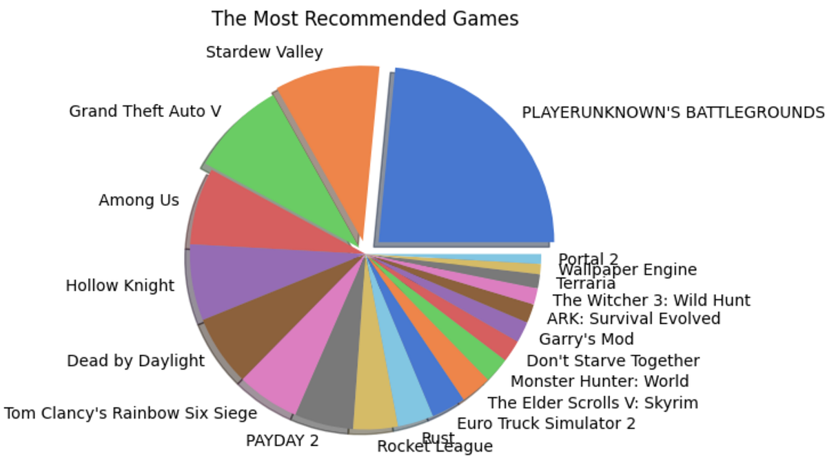
A complete guide to big data analysis using Apache Hadoop (HDFS) and PySpark library in Python on game reviews on the Steam gaming platform.With over 100 zettabytes (= 10¹²GB) of data produced every year around the world, the significance of handling big data is one of the most required skills today. Data Analysis, itself, could be defined as the ability to handle big data and derive insights from the never-ending and exponentially growing data. Apache Hadoop and Apache Spark are two of the basic tools that help us untangle the limitless possibilities hidden in large datasets. Apache Hadoop enables us to streamline data storage and distributed computing with its Distributed File System (HDFS) and the MapReduce-based parallel processing of data. Apache Spark is a big data analytics engine capable of EDA, SQL analytics, Streaming, Machine Learning, and Graph processing compatible with the major programming languages through its APIs. Both when combined form an exceptional environment for dealing with big data with the available computational resources — just a personal computer in most cases!Let us unfold the power of Big Data and Apache Hadoop with a simple analysis project implemented using Apache Spark in Python.To begin with, let's dive into the installation of Hadoop Distributed File System and Apache Spark on a MacOS. I am using a MacBook Air with macOS Sonoma with an M1 chip.Jump to the section —Installing Hadoop Distributed File SystemInstalling Apache SparkSteam Review Analysis using PySparkWhat next?1. Installing Hadoop Distributed File SystemThanks to Code With Arjun for the amazing article that helped me with the installation of Hadoop on my Mac. I seamlessly installed and ran Hadoop following his steps which I will show you here as well.a. Installing HomeBrewI use Homebrew for installing applications on my Mac for ease. It can be directly installed on the system with the below code —/bin/bash -c "$(curl -fsSL https://raw.githubusercontent.com/Homebrew/install/HEAD/install.sh)"Once it is installed, you can run the simple code below to verify the installation.brew --versionFigure 1: Image by AuthorHowever, you will likely encounter an error saying, command not found, this is because the homebrew will be installed in a different location (Figure 2) and it is not executable from the current directory. For it to function, we add a path environment variable for the brew, i.e., adding homebrew to the .bash_profile.Figure 2: Image by AuthorYou can avoid this step by using the full path to Homebrew in your commands, however, it might become a hustle at later stages, so not recommended!echo ‘eval “$(/opt/homebrew/bin/brew shellenv)”' >> /Users/rindhujajohnson/.bash_profileeval “$(/opt/homebrew/bin/brew shellenv)”Now, when you try, brew --version, it should show the Homebrew version correctly.b. Installing HadoopDisclaimer! Hadoop is a Java-based application and is supported by a Java Development Kit (JDK) version older than 11, preferably 8 or 11. Install JDK before continuing.Thanks to Code With Arjun again for this video on JDK installation on MacBook M1.https://medium.com/media/978a938e8d7a981d1b79b65db7884829/hrefNow, we install the Hadoop on our system using the brew command.brew install hadoopThis command should install Hadoop seamlessly. Similar to the steps followed while installing HomeBrew, we should edit the path environment variable for Java in the Hadoop folder. The environment variable settings for the installed version of Hadoop can be found in the Hadoop folder within HomeBrew. You can use which hadoop command to find the location of the Hadoop installation folder. Once you locate the folder, you can find the variable settings at the below location. The below command takes you to the required folder for editing the variable settings (Check the Hadoop version you installed to avoid errors).cd /opt/homebrew/Cellar/hadoop/3.3.6/libexec/etc/hadoopYou can view the files in this folder using the ls command. We will edit the hadoop-env.sh to enable the proper running of Hadoop on the system.Figure 3: Image by AuthorNow, we have to find the path variable for Java to edit the hadoop-ev.sh file using the following command./usr/libexec/java_homeFigure 4: Image by AuthorWe can open the hadoop-env.sh file in any text editor. I used VI editor, you can use any editor for the purpose. We can copy and paste the path — Library/Java/JavaVirtualMachines/adoptopenjdk-11.jdk/Contents/Home at the export JAVA_HOME = position.Figure 5: hadoop-env.sh file opened in VI Text EditorNext, we edit the four XML files in the Hadoop folder.core-site.xml<configuration> <property> <name>fs.defaultFS</name> <value>hdfs://localhost:9000</value> </property></configuration>hdfs-site.xml<configuration> <property> <name>dfs.replication</name> <value>1</value> </property></configuration>mapred-site.xml<configuration> <property> <name>mapreduce.framework.name</name> <value>yarn</value> </property> <property> <name>mapreduce.application.classpath</name> <value>$HADOOP_MAPRED_HOME/share/hadoop/mapreduce/*:$HADOOP_MAPRED_HOME/share/hadoop/mapreduce/lib/* </value> </property></configuration>yarn-site.xml<configuration> <property> <name>yarn.nodemanager.aux-services</name> <value>mapreduce_shuffle</value> </property> <property> <name>yarn.nodemanager.env-whitelist</name> <value>JAVA_HOME,HADOOP_COMMON_HOME,HADOOP_HDFS_HOME,HADOOP_CONF_DIR,CLASSPATH_PREPEND_DISTCACHE,HADOOP_YARN_HOME,HADOOP_MAPRED_HOME </value> </property></configuration>With this, we have successfully completed the installation and configuration of HDFS on the local. To make the data on Hadoop accessible with Remote login, we can go to Sharing in the General settings and enable Remote Login. You can edit the user access by clicking on the info icon.Figure 6: Enable Remote Access. Image by AuthorLet's run Hadoop!Execute the following commandshadoop namenode -format # starts the Hadoop environment% start-all.sh # Gathers all the nodes functioning to ensure that the installation was successful% jps Figure 7: Initiating Hadoop and viewing the nodes and resources running. Image by AuthorWe are all set! Now let's create a directory in HDFS and add the data will be working on. Let's quickly take a look at our data source and details.DataThe Steam Reviews Dataset 2021 (License: GPL 2) is a collection of reviews from about 21 million gamers covering over 300 different games in the year 2021. the data is extracted using Steam's API — Steamworks — using the Get List function.GET store.steampowered.com/appreviews/<appid>?json=1The dataset consists of 23 columns and 21.7 million rows with a size of 8.17 GB (that is big!). The data consists of reviews in different languages and a boolean column that tells if the player recommends the game to other players. We will be focusing on how to handle this big data locally using HDFS and analyze it using Apache Spark in Python using the PySpark library.c. Uploading Data into HDFSFirstly, we create a directory in the HDFS using the mkdir command. It will throw an error if we try to add a file directly to a non-existing folder.hadoop fs -mkdir /userhadoop fs - mkdir /user/steam_analysisNow, we will add the data file to the folder steam_analysis using the put command.hadoop fs -put /Users/rindhujajohnson/local_file_path/steam_reviews.csv /user/steam_analysisApache Hadoop also uses a user interface available at http://localhost:9870/.Figure 8: HDFS User Interface at localhost:9870. Image by AuthorWe can see the uploaded files as shown below.Figure 10: Navigating files in HDFS. Image by AuthorOnce the data interaction is over, we can use stop-all.sh command to stop all the Apache Hadoop daemons.Let us move to the next step — Installing Apache Spark2. Installing Apache SparkApache Hadoop takes care of data storage (HDFS) and parallel processing (MapReduce) of the data for faster execution. Apache Spark is a multi-language compatible analytical engine designed to deal with big data analysis. We will run the Apache Spark on Python in Jupyter IDE.After installing and running HDFS, the installation of Apache Spark for Python is a piece of cake. PySpark is the Python API for Apache Spark that can be installed using the pip method in the Jupyter Notebook. PySpark is the Spark Core API with its four components — Spark SQL, Spark ML Library, Spark Streaming, and GraphX. Moreover, we can access the Hadoop files through PySpark by initializing the installation with the required Hadoop version.# By default, the Hadoop version considered will be 3 here.PYSPARK_HADOOP_VERSION=3 pip install pysparkLet's get started with the Big Data Analytics!3. Steam Review Analysis using PySparkSteam is an online gaming platform that hosts over 30,000 games streaming across the world with over 100 million players. Besides gaming, the platform allows the players to provide reviews for the games they play, a great resource for the platform to improve customer experience and for the gaming companies to work on to keep the players on edge. We used this review data provided by the platform publicly available on Kaggle.3. a. Data Extraction from HDFSWe will use the PySpark library to access, clean, and analyze the data. To start, we connect the PySpark session to Hadoop using the local host address.from pyspark.sql import SparkSessionfrom pyspark.sql.functions import *# Initializing the Spark Sessionspark = SparkSession.builder.appName("SteamReviewAnalysis").master("yarn").getOrCreate()# Providing the url for accessing the HDFSdata = "hdfs://localhost:9000/user/steam_analysis/steam_reviews.csv"# Extracting the CSV data in the form of a Schemadata_csv = spark.read.csv(data, inferSchema = True, header = True)# Visualize the structure of the Schemadata_csv.printSchema()# Counting the number of rows in the datasetdata_csv.count() # 40,848,6593. b. Data Cleaning and Pre-ProcessingWe can start by taking a look at the dataset. Similar to the pandas.head() function in Pandas, PySpark has the SparkSession.show() function that gives a glimpse of the dataset.Before that, we will remove the reviews column in the dataset as we do not plan on performing any NLP on the dataset. Also, the reviews are in different languages making any sentiment analysis based on the review difficult.# Dropping the review column and saving the data into a new variabledata = data_csv.drop("review")# Displaying the datadata.show() Figure 11: The Structure of the SchemaWe have a huge dataset with us with 23 attributes with NULL values for different attributes which does not make sense to consider any imputation. Therefore, I have removed the records with NULL values. However, this is not a recommended approach. You can evaluate the importance of the available attributes and remove the irrelevant ones, then try imputing data points to the NULL values.# Drops all the records with NULL valuesdata = data.na.drop(how = "any")# Count the number of records in the remaining datasetdata.count() # 16,876,852We still have almost 17 million records in the dataset!Now, we focus on the variable names of the dataset as in Figure 11. We can see that the attributes have a few characters like dot(.) that are unacceptable as Python identifiers. Also, we change the data type of the date and time attributes. So we change these using the following code —from pyspark.sql.types import *from pyspark.sql.functions import from_unixtime# Changing the data type of each columns into appropriate typesdata = data.withColumn("app_id",data["app_id"].cast(IntegerType())). withColumn("author_steamid", data["author_steamid"].cast(LongType())). withColumn("recommended", data["recommended"].cast(BooleanType())). withColumn("steam_purchase", data["steam_purchase"].cast(BooleanType())). withColumn("author_num_games_owned", data["author_num_games_owned"].cast(IntegerType())). withColumn("author_num_reviews", data["author_num_reviews"].cast(IntegerType())). withColumn("author_playtime_forever", data["author_playtime_forever"].cast(FloatType())). withColumn("author_playtime_at_review", data["author_playtime_at_review"].cast(FloatType()))# Converting the time columns into timestamp data typedata = data.withColumn("timestamp_created", from_unixtime("timestamp_created").cast("timestamp")). withColumn("author_last_played", from_unixtime(data["author_last_played"]).cast(TimestampType())). withColumn("timestamp_updated", from_unixtime(data["timestamp_updated"]).cast(TimestampType()))Figure 12: A glimpse of the Steam review Analysis dataset. Image by AuthorThe dataset is clean and ready for analysis!3. c. Exploratory Data AnalysisThe dataset is rich in information with over 20 variables. We can analyze the data from different perspectives. Therefore, we will be splitting the data into different PySpark data frames and caching them to run the analysis faster.# Grouping the columns for each analysiscol_demo = ["app_id", "app_name", "review_id", "language", "author_steamid", "timestamp_created" ,"author_playtime_forever","recommended"]col_author = ["steam_purchase", 'author_steamid', "author_num_games_owned", "author_num_reviews", "author_playtime_forever", "author_playtime_at_review", "author_last_played","recommended"]col_time = [ "app_id", "app_name", "timestamp_created", "timestamp_updated", 'author_playtime_at_review', "recommended"]col_rev = [ "app_id", "app_name", "language", "recommended"]col_rec = ["app_id", "app_name", "recommended"]# Creating new pyspark data frames using the grouped columnsdata_demo = data.select(*col_demo)data_author = data.select(*col_author)data_time = data.select(*col_time)data_rev = data.select(*col_rev)data_rec = data.select(*col_rec)i. Games AnalysisIn this section, we will try to understand the review and recommendation patterns for different games. We will consider the number of reviews analogous to the popularity of the game and the number of True recommendations analogous to the gamer's preference for the game.Finding the Most Popular Games# the data frame is grouped by the game and the number of occurrences are countedapp_names = data_rec.groupBy("app_name").count()# the data frame is ordered depending on the count for the highest 20 gamesapp_names_count = app_names.orderBy(app_names["count"].desc()).limit(20)# a pandas data frame is created for plottingapp_counts = app_names_count.toPandas()# A pie chart is createdfig = plt.figure(figsize = (10,5))colors = sns.color_palette("muted")explode = (0.1,0.075,0.05,0,0,0,0,0,0,0,0,0,0,0,0,0,0,0,0,0)plt.pie(x = app_counts["count"], labels = app_counts["app_name"], colors = colors, explode = explode, shadow = True)plt.title("The Most Popular Games")plt.show()Finding the Most Recommended Games# Pick the 20 highest recommended games and convert it in to pandas data frametrue_counts = data_rec.filter(data_rec["recommended"] == "true").groupBy("app_name").count()recommended = true_counts.orderBy(true_counts["count"].desc()).limit(20)recommended_apps = recommended.toPandas()# Pick the games such that both they are in both the popular and highly recommended listtrue_apps = list(recommended_apps["app_name"])true_app_counts = data_rec.filter(data_rec["app_name"].isin(true_apps)).groupBy("app_name").count()true_app_counts = true_app_counts.orderBy(true_app_counts["count"].desc())true_app_counts = true_app_counts.toPandas()# Evaluate the percent of true recommendations for the top games and sort themtrue_perc = []for i in range(0,20,1): percent = (true_app_counts["count"][i]-recommended_apps["count"][i])/true_app_counts["count"][i]*100 true_perc.append(percent)recommended_apps["recommend_perc"] = true_percrecommended_apps = recommended_apps.sort_values(by = "recommend_perc", ascending = False)# Built a pie chart to visualizefig = plt.figure(figsize = (10,5))colors = sns.color_palette("muted")explode = (0.1,0.075,0.05,0,0,0,0,0,0,0,0,0,0,0,0,0,0,0,0,0)plt.pie(x = recommended_apps["recommend_perc"], labels = recommended_apps["app_name"], colors = colors, explode = explode, shadow = True)plt.title("The Most Recommended Games")plt.show()Figure 13: Shows the pie charts for popular and recommended games. Images by AuthorInsightsPlayer Unknown's Battlegrounds (PUBG) is the most popular and most recommended game of 2021.However, the second positions for the two categories are held by Grand Theft Auto V (GTA V) and Stardew Valley respectively. This shows that being popular does not mean all the players recommend the game to another player.The same pattern is observed with other games also. However, the number of reviews for a game significantly affects this trend.ii. Demographic AnalysisWe will find the demography, especially, the locality of the gamers using the data_demo data frame. This analysis will help us understand the popular languages used for review and languages used by reviewers of popular games. We can use this trend to determine the demographic influence and sentiments of the players to be used for recommending new games in the future.Finding Popular Review Languages# We standardize the language names in the language column, then group them,# Count by the groups and convert into pandas df after sorting them the countauthor_lang = data_demo.select(lower("language").alias("language")) .groupBy("language").count().orderBy(col("count").desc()). limit(20).toPandas()# Plotting a bar graphfig = plt.figure(figsize = (10,5))plt.bar(author_lang["language"], author_lang["count"])plt.xticks(rotation = 90)plt.xlabel("Popular Languages")plt.ylabel("Number of Reviews (in Millions)")plt.show()Finding Review Languages of Popular Games# We group the data frame based on the game and language and count each occurrencedata_demo_new = data_demo.select(lower("language"). alias("language"), "app_name")games_lang = data_demo_new.groupBy("app_name","language").count().orderBy(col("count").desc()).limit(100).toPandas()# Plot a stacked bar graph to visualizegrouped_games_lang = games_lang_df.pivot(index='app_name', columns='language', values='count')grouped_games_lang.plot(kind='bar', stacked=True, figsize=(12, 6))plt.title('Count of Different App Names and Languages')plt.xlabel('App Name')plt.ylabel('Count')plt.show()Figure 14: Language Popularity; Language Popularity among Popular games. Images by AuthorInsightsEnglish is the most popular language used by reviewers followed by Schinese and RussianSchinese is the most widely used language for the most popular game (PUBG), whereas, English is widely used for the second most popular game (GTA V) and almost all others!The popularity of a game seems to have roots in the area of origin. PUBG is a product of a South Korean gaming company and we observe that it has the Korean language among one of the highly used.Time, author, and review analyses are also performed on this data, however, do not give any actionable insights. Feel free to visit the GitHub repository for the full project documentation.3. d. Game Recommendation using Spark ML LibraryWe have reached the last stage of this project, where we will implement the Alternating Least Squares (ALS) machine-learning algorithm from the Spark ML Library. This model utilizes the collaborative filtering technique to recommend games based on player's behavior, i.e., the games they played before. This algorithm identifies the game selection pattern for players who play each available game on the Steam App.For the algorithm to work,We require three variables — the independent variable, target variable(s) — depending on the number of recommendations, here 5, and a rating variable.We encode the games and the authors to make the computation easier. We also convert the booleanrecommended column into a rating column with True = 5, and False = 1.Also, we will be recommending 5 new games for each played game and therefore we consider the data of the players who have played more than five for modeling the algorithm.Let's jump to the modeling and recommending part!new_pair_games = data_demo.filter(col("author_playtime_forever")>=5*mean_playtime)new_pair_games = new_pair_games.filter(new_pair_games["author_steamid"]>=76560000000000000).select("author_steamid","app_id", "app_name","recommended")# Convert author_steamid and app_id to indices, and use the recommended column for ratingauthor_indexer = StringIndexer(inputCol="author_steamid", outputCol="author_index").fit(new_pair_games)app_indexer = StringIndexer(inputCol="app_name", outputCol="app_index").fit(new_pair_games)new_pair_games = new_pair_games.withColumn("Rating", when(col("recommended") == True, 5).otherwise(1))# We apply the indexing to the data frame by invoking the reduce phase function transform()new_pair = author_indexer.transform(app_indexer.transform(new_pair_games))new_pair.show()# The reference chart for gamesgames = new_pair.select("app_index","app_name").distinct().orderBy("app_index")Figure 16: The game list with the corresponding index for reference. Image by AuthorImplementing ALS Algorithm# Create an ALS (Alternating Least Squares) modelals = ALS(maxIter=10, regParam=0.01, userCol="app_index", itemCol="author_index", ratingCol="Rating", coldStartStrategy="drop")# Fit the model to the datamodel = als.fit(new_pair)# Generate recommendations for all itemsapp_recommendations = model.recommendForAllItems(5) # Number of recommendations per item# Display the recommendationsapp_recommendations.show(truncate=False)Figure 17: The recommendation and rating generated for each author based on their gaming history. Image by AuthorWe can cross-match the indices from Figure 16 to find the games recommended for each player. Thus, we implemented a basic recommendation system using the Spark Core ML Library.3. e. ConclusionIn this project, we could successfully implement the following —Download and install the Hadoop ecosystem — HDFS and MapReduce — to store, access, and extract big data efficiently, and implement big data analytics much faster using a personal computer.Install the Apache Spark API for Python (PySpark) and integrate it with the Hadoop ecosystem, enabling us to carry out big data analytics and some machine-learning operations.The games and demographic analysis gave us some insights that can be used to improve the gaming experience and control the player churn. Keeping the players updated and informed about the trends in their peers should be a priority for the Steam platform. Suggestions like “most played”, “most played in your region”, “most recommended”, and “don't miss out on these new games” can keep the players active.The Steam Application can use the ALS recommendation system to recommend new games to existing players based on their profile and keep them engaged and afresh.4. What Next?Implement Natural Language Processing techniques in the review column, for different languages to extract the essence of the reviews and improve the gaming experience.Steam can report bugs in the games based on the reviews. Developing an AI algorithm that captures the review content, categorizes it, and sends it to appropriate personnel could do wonders for the platform.Comment what you think can be done more!5. ReferencesApache Hadoop. Apache Hadoop. Apache HadoopStatista. (2021). Volume of data/information created, captured, copied, and consumed worldwide from 2010 to 2020, with forecasts from 2021 to 2025 statistaDey, R. (2023). A Beginner's Guide to Big Data and Hadoop Distributed File System (HDFS). MediumCode with Arjun (2021). Install Hadoop on Mac OS (MacBook M1). MediumApache Spark. PySpark Installation. Apache SparkApache Spark. Collaborative Filtering with ALS). Apache SparkLet's Uncover it. (2023). PUBG. Let's Uncover ItYou can find the complete big data analysis project in my GitHub repository.Let's connect on LinkedIn and discuss more!If you found this article useful, clap, share, and comment!Apache Hadoop and Apache Spark for Big Data Analysis was originally published in Towards Data Science on Medium, where people are continuing the conversation by highlighting and responding to this story.

A l'occasion de l'évènement « Let Loose », Apple a lancé sa nouvelle puce M4. Cette dernière se focalise davantage … Cet article Apple dévoile la puce M4 ! Bienvenu dans l'ère des iPhones dopés à l'IA a été publié sur LEBIGDATA.FR.

Ofcom is cracking down on Instagram, YouTube and 150,000 other web services to improve child safety online. A new Children’s Safety Code from the U.K. Internet regulator will push tech firms to run better age checks, filter and downrank content, and apply around 40 other steps to assess harmful content around subjects like suicide, self […] © 2024 TechCrunch. All rights reserved. For personal use only.

Reduce dimensionality and cluster Taipei MRT stations based on hourly trafficTaipei Rail Map ( Actually Introduced Romanization Standards based ) Including THSR, TRA, Taipei MRT & Other Lines. Image by Taiwan J.Principal Component Analysis (PCA) has been used in traffic data to detect anomalies, but it can also be used to capture the patterns of a transit station's traffic history, just like what it does on the purchase data of a customer.In this article, we will go through:What tricks does PCA doWhat can we do after applying PCAPlaytime! Take a look into our dataset: Taipei Metro Rapid Transit System, Hourly Traffic DataUsing PCA on hourly traffic dataClustering on the PCA resultInsights on the Taipei MRT trafficKey takeaways1. What tricks does PCA doIn brief, PCA summarizes the data by finding linear combinations of features, which can be thought of as taking several pictures of an 3D object, and it will naturally sort the pictures by the most representative to the least before handing to you.WIth the input being our original data, there would be 2 useful outputs of PCA: Z and W. By multiply them, we can get the reconstruction data, which is the original data but with some tolerable information loss (since we have reduced the dimensionality.)We will explain these 2 output matrices with our data in the practice below.2. What can we do after applying PCAAfter apply PCA to our data to reduce the dimensionality, we can use it for other machine learning tasks, such as clustering, classification, and regression.In the case of Taipei MRT later in this artical, we will perform clustering on the lower dimensional data, where a few dimensions can be interpreted as passenger proportions in different parts of a day, such as morning, noon, and evening. Those stations share similar proportions of passengers in the daytime would be consider to be in the same cluster (their patterns are alike!).3. Take a look in our traffic dataset!The datast we use here is Taipei Metro Rapid Transit System, Hourly Traffic Data, with columns: date, hour, origin, destination, passenger_count.In our case, I will keep weekday data only, since there are more interesting patterns between different stations during weekdays, such as stations in residential areas may have more commuters entering in the daytime, while in the evening, those in business areas may have more people getting in.Stations in residential areas may have more commuters entering in the daytime.The plot above is 4 different staitons' hourly traffic trend (the amount the passengers entering into the station). The 2 lines in red are Xinpu and Yongan Market, which are actually located in the super crowded areas in New Taipei City. On the otherhands, the 2 lines in blue are Taipei City Hall and Zhongxiao Fuxing, where most of the companies located and business activities happen.The trends reflect both the nature of these areas and stations, and we can notice that the difference is most obvious when comparing their trends during commute hours (7 to 9 a.m., and 17 to 19 p.m.).4. Using PCA on hourly traffic dataWhy reducing dimensionality before conducting further machine learning tasks?There are 2 main reasons:As the number of dimensions increases, the distance between any two data points becomes closer, and thus more similar and less meaningful, which would be refered to as “the curse of dimensionality”.Due to the high-dimensional nature of the traffic data, it is difficult to visualize and interpret.By applying PCA, we can identify the hours when the traffic trends of different stations are most obvious and representative. Intuitively, by the plot shown previously, we can assume that hours around 8 a.m. and 18 p.m. may be representative enough to cluster the stations.Remember we mentioned the useful output matrices, Z and W, of PCA in the previous section? Here, we are going to interpret them with our MRT case.Original data, XIndex : starionsColumn : hoursValues : the proportion of passenger entering in the specific hour (#passenger / #total passengers)With such X, we can apply PCA by the following code:from sklearn.decomposition import PCAn_components = 3pca = PCA(n_components=n_components)X_tran = StandardScaler().fit_transform(X)pca = PCA(n_components=n_components, whiten=True, random_state=0)pca.fit(X_tran)Here, we specify the parameter n_components to be 3, which implies that PCA will extract the 3 most significant components for us.Note that, it is like “taking several pictures of an 3D object, and it will sort the pictures by the most representative to the least,” and we choose the top 3 pictures. So, if we set n_components to be 5, we will get 2 more pictures, but our top 3 will remain the same!PCA output, W matrixW can be thought of as the weights on each features (i.e. hours) with regard to our “pictures”, or more specificly, principal components.pd.set_option('precision', 2)W = pca.components_W_df = pd.DataFrame(W, columns=hour_mapper.keys(), index=[f'PC_{i}' for i in range(1, n_components+1)])W_df.round(2).style.background_gradient(cmap='Blues')For our 3 principal components, we can see that PC_1 weights more on night hours, while PC_2 weights more on noon, and PC_3 is about morning time.PCA output, Z matrixWe can interpret Z matrix as the representations of stations.Z = pca.fit_transform(X)# Name the PCs according to the insights on W matrixZ_df = pd.DataFrame(Z, index=origin_mapper.keys(), columns=['Night', 'Noon', 'Morning'])# Look at the stations we demonstrated earlierZ_df = Z_df.loc[['Zhongxiao_Fuxing', 'Taipei_City_Hall', 'Xinpu', 'Yongan_Market'], :]Z_df.style.background_gradient(cmap='Blues', axis=1)In our case, as we have interpreted the W matrix and understand the latent meaning of each components, we can assign the PCs with names.The Z matrix for these 4 stations indicates that the first 2 stations have larger proportion of night hours, while the other 2 have more in the mornings. This distribution also seconds the findings in our EDA (recall the line chart of these 4 stations in the earlier part).5. Clustering on the PCA result with K-MeansAfter getting the PCA result, let's further cluster the transit stations according to their traffic patterns, which is represented by 3principal components.In the last section, Z matrix has representations of stations with regard to night, noon, and morning.We will cluster the stations based on these representations, such that the stations in the same group would have similar passenger distributions among these 3 periods.There are bunch of clustering methods, such as K-Means, DBSCAN, hierarchical clustering, e.t.c. Since the main topic here is to see the convenience of PCA, we will skip the process of experimenting which method is more suitable, and go with K-Means.from sklearn.cluster import KMeans# Fit Z matrix to K-Means model kmeans = KMeans(n_clusters=3)kmeans.fit(Z)After fitting the K-Means model, let's visualize the clusters with 3D scatter plot by plotly.import plotly.express as pxcluster_df = pd.DataFrame(Z, columns=['PC1', 'PC2', 'PC3']).reset_index()# Turn the labels from integers to strings, # such that it can be treated as discrete numbers in the plot.cluster_df['label'] = kmeans.labels_cluster_df['label'] = cluster_df['label'].astype(str)fig = px.scatter_3d(cluster_df, x='PC1', y='PC2', z='PC3', color='label', hover_data={"origin": (pca_df['index'])}, labels={ "PC1": "Night", "PC2": "Noon", "PC3": "Morning", }, opacity=0.7, size_max=1, width = 800, height = 500 ).update_layout(margin=dict(l=0, r=0, b=0, t=0) ).update_traces(marker_size = 5)6. Insights on the Taipei MRT traffic — Clustering resultsCluster 0 : More passengers in daytime, and therefore it may be the “living area” group.Cluster 2 : More passengers in evening, and therefore it may be the “business area” group.Cluster 1 : Both day and night hours are full of people entering the stations, and it is more complicated to explain the nature of these stations, for there could be variant reasons for different stations. Below, we will take a look into 2 extreme cases in this cluster.For example, in Cluster 1, the station with the largest amount of passengers, Taipei Main Station, is a huge transit hub in Taipei, where commuters are allowed to transfer from buses and railway systems to MRT here. Therefore, the high-traffic pattern during morning and evening is clear.On the contrary, Taipei Zoo station is in Cluster 1 as well, but it is not the case of “both day and night hours are full of people”. Instead, there is not much people in either of the periods because few residents live around that area, and most citizens seldom visit Taipei Zoo on weekdays.The patterns of these 2 stations are not much alike, while they are in the same cluster. That is, Cluster 1 might contain too many stations that are actually not similar. Thus, in the future, we would have to fine-tune hyper-parameters of K-Means, such as the number of clusters, and methods like silhouette score and elbow method would be helpful.ConclusionIn summary,Applying PCA on traffic data to reduce dimensionality can be implemented as extracting 3 important periods (morning, noon, evening) from totally 21 working hours.PCA outputs are W and Z matrices, where Z can be viewed as the representations of stations with regard to principal components (time periods), and W can be thought of as the representations of principal components (time periods) with regard to original features (hours).Considering W matrix can help us understand the latent meaning of each principal component.Clustering methods can be used on the PCA output, Z matrix.Note that we skipped EDA and hyper-parameters tuning here in order to focus on the topic of this article, but they are actually important.Thank you for reading so far! Hope you have a wonderful online journey in Taipei 🫶Further ReadingsKMeans Hyper-parameters Explained with Examples, Sujeewa Kumaratunga PhDHow to Combine PCA and K-means Clustering in Python?, Elitsa KaloyanovaReferenceDSCI 563 Lecture Notes, UBC Master of Data Science, Varada KolhatkarK Means Clustering on High Dimensional Data., shivangi singhCurse of Dimensionality — A “Curse” to Machine Learning, Shashmi KaranamUnless otherwise noted, all images are by the author.PCA & K-Means for Traffic Data in Python was originally published in Towards Data Science on Medium, where people are continuing the conversation by highlighting and responding to this story.

A data-driven approachContinue reading on Towards Data Science »

C'est maintenant autour des docteurs de s'inquiéter pour leur travail à cause de Med-Gemini. La précision de ses diagnostics cliniques … Cet article Google a créé une IA docteur, et elle va envoyer votre médecin chez France Travail a été publié sur LEBIGDATA.FR.

Meta claims that it has strong guardrails in place to prevent its system from generating inappropriate ad content or low-quality images. © 2024 TechCrunch. All rights reserved. For personal use only.

Robert Kahn has been a consistent presence on the Internet since its creation — obviously, since he was its co-creator. But like many tech pioneers his resumé is longer than that and in fact his work prefigured such ostensibly modern ideas as AI agents and blockchain. TechCrunch chatted with Kahn about how, really, nothing has […] © 2024 TechCrunch. All rights reserved. For personal use only.

Amazon is launching a new tool, Bedrock Studio, designed to let organizations experiment with generative AI models, collaborate on those models, and ultimately build generative AI-powered apps. Available in public preview starting today, the web-based Bedrock Studio — a part of Bedrock, Amazon’s generative AI tooling and hosting platform — provides what Amazon describes in […] © 2024 TechCrunch. All rights reserved. For personal use only.