Toute l'actualité de l'IA et du Big data
Learn Shiny for Python with a Puppy Traits Dashboard
Step-by-step guide to creating “Who is the Goodest Doggy” Application with Shiny for Python, from foundation to styling.Continue reading on Towards Data Science »
Learn Shiny for Python with a Puppy Traits Dashboard...
Step-by-step guide to creating “Who is the Goodest Doggy” Application...
Source: Towards Data Science
The Math Behind Batch Normalization
Explore Batch Normalization, a cornerstone of neural networks, understand its mathematics and implement it from scratch.Continue reading on Towards Data Science »
The Math Behind Batch Normalization
Explore Batch Normalization, a cornerstone of neural networks, understand its mathematics...
Source: Towards Data Science
Samsung Medison to acquire French AI ultrasound startup Sonio for .7M

The French startup's AI assistant is aimed at helping obstetricians and gynecologists with the evaluation and documentation of ultrasound exams. © 2024 TechCrunch. All rights reserved. For personal use only.
Samsung Medison to acquire French AI ultrasound startup...
The French startup's AI assistant is aimed at helping obstetricians and gynecologists...
Source: TechCrunch AI News
The struggle of Artificially Imitated Intelligence in specialist domains
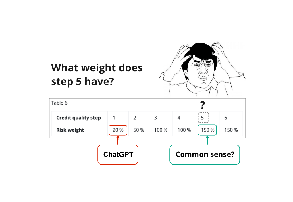
And why the path to real intelligence goes through ontologies and knowledge graphsThose who follow me, might remember a similar AI rant from a year ago, under the pseudonym “Grumpy Risk Manager”. Now I'm back, grumpier than ever, with specific examples but also ideas for solutions!Source: author collageIntroductionLarge Language Models (LLMs) like ChatGPT are impressive in their ability to discuss generic topics in natural language.However, they struggle in specialist domains such as medicine, finance and law.This is due to lack of real understanding and focus on imitation rather than intelligence.LLMs are at the peak of their hype. They are considered “intelligent” due to their ability to answer and discuss generic topics in natural language.However, once you dive into a specialist/complex domains such as medicine, finance, law, it is easy to observe logical inconsistencies, plain mistakes and the so called “hallucinations”. To put it simply, the LLM behaves like a pupil with a very rich dictionary who tries to pretend that they've studied for the exam and know all the answers, but they actually don't! They just pretend to be intelligent due to the vast information at their disposal, but their ability to reason using this information is very limited. I would even go a step further and say that:The so-called Artificial Intelligence (AI) is very often Artificial Imitation of Intelligence (AII). This is particularly bad in specialist domains like medicine or finance, since a mistake there can lead to human harm and financial losses.Let me give you a real example from the domain in which I've spent the last 10 years — financial risk. Good evidence of it being “specialist” is the amount of contextual information that has to be provided to the average person in order to understand the topic:Banks are subject to regulatory Capital requirements.Capital can be considered a buffer which absorbs financial losses.The requirements to hold Capital, ensures that banks have sufficient capability to absorb losses reducing the likelihood of bankruptcy and financial crisis.The rules for setting the requirements in 1. are based on risk-proportionality principles:→ the riskier the business that banks undertake→ higher risk-weights→ higher capital requirements→ larger loss buffer→ stable bankThe degree of riskiness in 4. is often measured in the form of credit rating of the firms with which the bank does business.Credit ratings come from different agencies and in different formats.In order to standardise the ratings, regulators have created mapping rules from every rating format to the standardised Credit Quality Step (CQS) in the range of 1 to 6.Then the regulatory rules for determining the risk-weights in 4. are based on the CQS.The rules in 8. for European banks are set in the Capital Requirements Regulation (CRR).The topic in the 9 statements above seems complex and it really is, there are dozens of additional complications and cases that exist, but which I've avoided on purpose, as they are not even necessary for illustrating the struggle of AII with such topics. Furthermore, the complexity doesn't arise from any of the individual 9 rules itself, but rather from their combination, there are a lot of concepts whose definition is based on several other concepts giving rise to a semantic net/graph of relationships connecting the concepts and the rules.Now let's focus only on the core concepts and rules in 4, which can be summarised as follows: rating → CQS → risk-weight → capital requirement. If we also look at an example CRR article 122, we can see a mapping table CQS → risk-weight which should be used for corporate exposures.Capital Requirements Regulation (CRR 122)This mapping rule is very simple, it can be understood easily by the average person with a bit of context. It is also known by many banking specialists and most of them don't memorise the exact rule but simply know the information of the 9 statements above and know where to look in order to see the exact mapping.Artificially Imitated IntelligenceNow let's formulate a question and see whether AII can deal with it, here is what I asked ChatGPT 3.5:According to CRR, what is the risk-weight of an exposure to corporate which has credit quality step of 5?And here is the answer:In the Capital Requirements Regulation (CRR), the risk-weight of an exposure to a corporate entity depends on its credit quality step. In the context of credit quality steps, a credit quality step of 5 typically represents the highest credit quality, indicating a very low risk of default.In the standardised approach outlined in the CRR, exposures to corporates are assigned risk weights based on their credit ratings or credit quality steps. The risk weights for exposures to corporates range from 20% to 150%, depending on the credit quality step and whether the exposure is short-term or long-term.Since a credit quality step of 5 signifies a very low risk, the corresponding risk weight assigned to such an exposure would be one of the lowest. In this case, for a corporate with a credit quality step of 5, the risk weight would likely be 20% or similar, indicating a low capital requirement for banks holding such exposures.Can you spot the factual mistakes, highlighted in bold?First very big mistake is that the AII completely misunderstood and inverted the CQS → risk-weight relationship, high CQS of 5 doesn't represent low risk but exactly the opposite, it is one of the highest risks! This is actually the biggest mistake one could possibly make when answering this question!Even after the mistake in 1, I would expect the AII to be able to look-up a table in an article and conclude that below a CQS of 5, there is a risk-weight of 150%. But no, the AII confidently claims 20% risk-weight, due to low risk…Although undeserved, I still gave the benefit of doubt to the AII, by asking the same question but clarifying the exact CRR article: 122. Shameless, but confident, the AII now responded that the risk-weight should be 100%, still claiming that CQS of 5 is good credit quality → another obvious mistake.Feeling safe for my job and that the financial industry still needs me, I started thinking about solutions, which ironically could make my job unsafe in the future…Why ontologies and knowledge graphs?Enter ontologies, a form of knowledge representation of a particular domain. One good way of thinking about it, is in terms of ordering the different ways of representing knowledge from least to more sophisticated:Data dictionary: table with field names and metadata attributesTaxonomy: table/s with added nesting of data types and sub-types in terms of relationships (e.g. Pigeon <is a type of> Bird)Ontology: Multidimensional taxonomies with more than one type of relationships (e.g. Birds <eat> Seeds) “the unholy marriage of a taxonomy with object oriented programming” (Kurt Cagle, 2017)Why would one want to incorporate such complex relational structure in their data? Below are the benefits which will be later illustrated with an example:Uniform representation of: structure, data and logic. In the example above, Bird is a class which is a template with generic properties = structure. In an ontology, we can also define many actual instances of individual Birds with their own properties = data. Finally, we can also add logic (e.g. If a Bird <eats> more than 5 Seeds, then <it is> not Hungry). This is essentially making the data “smart” by incorporating some of the logic as data itself, thus making it a reusable knowledge. It also makes information both human and machine readable which is particularly useful in ML.Explainability and Lineage: most frequent implementation of ontology is via Resource Description Framework (RDF) in the form of graphs. These graphs can then be queried in order to evaluate existing rules and instances or add new ones. Moreover, the chain of thought, through the graph nodes and edges can be traced, explaining the query results and avoiding the ML black box problem.Reasoning and Inference: when new information is added, a semantic reasoner can evaluate the consequences on the graph. Moreover, new knowledge can be derived from existing one via “What if” questions.Consistency: any conflicting rules or instances that deviate from the generic class properties are automatically identified as an error by the reasoner and cannot become part of the graph. This is extremely valuable as it enforces agreement of knowledge in a given area, eliminating any subjective interpretations.Interoperability and Scalability: the reusable knowledge can focus on a particular specialist domain or connect different domains (see FIBO in finance, OntoMathPRO in maths, OGMS in medicine). Moreover, one could download a general industry ontology and extend it with private enterprise data in the form of instances and custom rules.Ontologies can be considered one of the earliest and purest forms of AI, long before large ML models became a thing and all based on the idea of making data smart via structuring. Here by AI, I mean real intelligence — the reason the ontology can explain the evaluated result of a given rule is because it has semantic understanding about how things work! The concept became popular first under the idea of Semantic Web in the early 2000s, representing the evolution of the internet of linked data (Web 3.0), from the internet of linked apps (Web 2.0) and the internet of linked pages (Web 1.0).Knowledge Graphs (KGs) are a bit more generic term for the storage of data in graph format, which may not necessarily follow ontological and semantic principles, while the latter are usually represented in the form of a KG. Nowadays, with the rise of LLMs, KGs are often seen as a good candidate for resolving their weaknesses in specialist domains, which in turn revives the concept of ontologies and their KG representation.This leads to very interesting convergence of paradigms:Ontologies aim to generate intelligence through making the data smart via structure.LLMs aim to generate intelligence through leaving the data unstructured but making the model very large and structural: ChatGPT has around 175 billion parameters!Clearly the goal is the same, and the outcome of whether the data becomes part of the model or the model becomes part of the data becomes simply a matter of reference frame, inevitably leading to a form of information singularity.Why use ontologies in banking?Specialisation: as shown above, LLMs struggle in specialist fields such as finance. This is particularly bad in a field in which mistakes are costly. In addition, value added from automating knowledge in specialist domains that have fewer qualified experts can be much higher than that of automation in generic domains (e.g. replacing banking expert vs support agent).Audit trail: when financial items are evaluated and aggregated in a financial statement, regulators and auditors expect to have continuous audit trail from all granular inputs and rules to the final aggregate result.Explainability: professionals rely on having a good understanding of the mechanisms under which a bank operates and impact of risk drivers on its portfolios and business decisions. Moreover, regulators explicitly require such understanding via regular “What if” exercises in the form of stress testing. This is one of the reasons ML has seen poor adoption in core banking — the so-called black box problem.Objectivity and Standardisation: lack of interpretation and subjectivity ensures level playing field in the industry, fair competition and effectiveness of the regulations in terms of ensuring financial stability.Now imagine a perfect world in which regulations such as the CRR are provided in the form of ontology rather than free text.Each bank can import the ontology standard and extend it with its own private data and portfolio characteristics, and evaluate all regulatory rules.Furthermore, the individual enterprise strategy can be also combined with the regulatory constraints in order to enable automated financial planning and optimised decision making.Finally, the complex composite impacts of the big graph of rules and data can be disentangled in order to explain the final results and give insights into previously non-obvious relationships.The below example aims to illustrate these ideas on a minimal effort, maximum impact basis!ExampleOn the search for solutions of the illustrated LLM weaknesses, I designed the following example:Create an ontology in the form of a knowledge graph.Define the structure of entities, add individual instances/data and logic governing their interactions, following the CRR regulation.Use the knowledge graph to evaluate the risk-weight.Ask the KG to explain how it reached this result.For creating the simple ontology, I used the CogniPy library with the main benefits of:Using Controlled Natural Language (CNL) for both writing and querying the ontology, meaning no need to know specific graph query languages.Visualisation of the materialised knowledge graphs.Reasoners with ability to explain results.StructureFirst, let's start by defining the structure of our ontology. This is similar to defining classes in objective oriented programming with different properties and constraints.In the first CNL statement, we define the company class and its properties.Every company has-id one (some integer value) and has-cqs one (some integer value) and has-turnover (some double value).Several things to note is that class names are with small letter (company). Different relationships and properties are defined with dash-case, while data types are defined in the brackets. Gradually, this starts to look more and more like a fully fledged programming language based on plain English.Next, we illustrate another ability to denote the uniqueness of the company based on its id via generic class statement.Every X that is a company is-unique-if X has-id equal-to something.DataNow let's add some data or instances of the company class, with instances starting with capital letter.Lamersoft is a company and has-id equal-to 123 and has-cqs equal-to 5 and has-turnover equal-to 51000000.Here we add a data point with a specific company called Lamersoft, with assigned values to its properties. Of course, we are not limited to a single data point, we could have thousands or millions in the same ontology and they can be imported with or without the structure or the logic components.Now that we've added data to our structure, we can query the ontology for the first time to get all companies, which returns a DataFrame of instances matching the query:onto.select_instances_of("a thing that is a company")DataFrame with query resultsWe can also plot our knowledge graph, which shows the relationship between the Lamersoft instance and the general class company:onto.draw_graph(layout='hierarchical')Ontology graphLogicFinally, let's add some simple rules implementing the CRR risk-weight regulations for corporates.If a company has-turnover greater-than 50000000 then the company is a corporate.If a corporate has-cqs equal-to 5 then the corporate has-risk-weight equal-to 1.50.The first rule defines what a corporate is, which usually is a company with large turnover above 50 million. The second rule implements part of the CRR mapping table CQS → risk-weight which was so hard to understand by the LLM.After adding the rules, we've completed our ontology and can plot the knowledge graph again:Ontology graph with evaluated rulesNotably, 2 important deductions have been made automatically by the knowledge graph as soon as we've added the logic to the structure and data:Lamersoft has been identified as a corporate due to its turnover property and the corporate classification rule.Lamersoft's risk-weight has been evaluated due to its CQS property and the CRR rule.This is all as a result of the magical automated consistency (no conflicts) of all information in the ontology. If we were to add any rule or instance that contradicts any of the existing information we would get an error from the reasoner and the knowledge graph would not be materialised.Now we can also play with the reasoner and ask why a given evaluation has been made or what is the chain of thought and audit trail leading to it:printWhy(onto,"Lamersoft is a corporate?"){ "by": [ { "expr": "Lamersoft is a company." }, { "expr": "Lamersoft has-turnover equal-to 51000000." } ], "concluded": "Lamersoft is a corporate.", "rule": "If a company has-turnover greater-than 50000000 then the company is a corporate."}Regardless of the output formatting, we can still clearly read that by the two expressions defining Lamersoft as a company and its specific turnover, it was concluded that it is a corporate because of the specific turnover condition. Unfortunately, the current library implementation doesn't seem to support an explanation of the risk-weight result, which is food for the future ideas section.Nevertheless, I deem the example successful as it managed to unite in a single scalable ontology, structure, data and logic, with minimal effort and resources, using natural English. Moreover, it was able to make evaluations of the rules and explain them with a complete audit trail.One could say here, ok what have we achieved, it is just another programming language closer to natural English, and one could do the same things with Python classes, instances and assertions. And this is true, to the extent that any programming language is a communication protocol between human and machine. Also, we can clearly observe the trend of the programming syntaxes moving closer to the human language, from the Domain Driven Design (DDD) focusing on implementing the actual business concepts and interactions, to the LLM add-ons of Integrated Development Environments (IDEs) to generate code from natural language. This becomes a clear trend:The role of programmers as intermediators between the business and the technology is changing. Do we need code and business documentation, if the former can be generated directly from the natural language specification of the business problem, and the latter can be generated in the form of natural language definition of the logic by the explainer?ConclusionImagine a world in which all banking regulations are provided centrally by the regulator not in the form of text but in the form of an ontology or smart data, that includes all structure and logic. While individual banks import the central ontology and extend it with their own data, thus automatically evaluating all rules and requirements. This will remove any room for subjectivity and interpretation and ensure a complete audit trail of the results.Beyond regulations, enterprises can develop their own ontologies in which they encode, automate and reuse the knowledge of their specialists or different calculation methodologies and governance processes. On an enterprise level, such ontology can add value for enforcing a common dictionary and understanding of the rules and reduce effort wasted on interpretations and disagreements which can be redirected to building more knowledge in the form of ontology. The same concept can be applied to any specialist area in which:Text association is not sufficient and LLMs struggle.Big data for effective ML training is not available.Highly-qualified specialists can be assisted by real artificial intelligence, reducing costs and risks of mistakes.If data is nowadays deemed as valuable as gold, I believe that the real diamond is structured data, that we can call knowledge. Such knowledge in the form of ontologies and knowledge graphs can also be traded between companies just like data is traded now for marketing purposes. Who knows, maybe this will evolve into a pay-per-node business model, where expertise in the form of smart data can be sold as a product or service.Then we can call intelligence our ability to accumulate knowledge and to query it for getting actionable insights. This can evolve into specialist AIs that tap into ontologies in order to gain expertise in a given field and reduce hallucinations.LLMs are already making an impact on company profits — Klarna is expected to have million improvement on profits as a result of ChatGPT handling most of its customer service chats, reducing the costs for human agents.Note however the exact area of application of the LLM! This is not the more specialised fields of financial/product planning or asset and liabilities management of a financial company such as Klarna. It is the general customer support service, which is the entry level position in many companies, which already uses a lot of standardised responses or procedures. The area in which it is easiest to apply AI but also in which the value added might not be the largest. In addition, the risk of LLM hallucination due to lack of real intelligence is still there. Especially in the financial services sector, any form of “financial advice” by the LLM can lead to legal and regulatory repercussions.Future ideasLLMs already utilise knowledge graphs in the so-called Retrieval-Augmented Generation (RAG). However, these graphs are generic concepts that might include any data structure and do not necessarily represent ontologies, which use by LLMs is relatively less explored. This gives me the following ideas for next article:Use plain English to query the ontology, avoiding reliance on particular CNL syntax — this can be done via NLP model that generates queries to the knowledge graph in which the ontology is stored — chatting with KGs.Use a more robust way of generating the ontology — the CogniPy library was useful for quick illustration, however, for extended use a more proven framework for ontology-oriented programming should be used like Owlready2.Point 1. enables the general user to get information from the ontology without knowing any programming, however, point 2 implies that a software developer is needed for defining and writing to the ontology (which has its pros and cons). However, if we want to close the AI loop, then specialists should be able to define ontologies using natural language and without the need for developers. This will be harder to do, but similar examples already exist: LLM with KG interface, entity resolution.A proof of concept that achieves all 3 points above can claim the title of true AI, it should be able to develop knowledge in a smart data structure which is both human and machine readable, and query it via natural language to get actionable insights with complete transparency and audit trail.Follow me for part 2!The struggle of Artificially Imitated Intelligence in specialist domains was originally published in Towards Data Science on Medium, where people are continuing the conversation by highlighting and responding to this story.
The struggle of Artificially Imitated Intelligence...
And why the path to real intelligence goes through ontologies and knowledge graphsThose...
Source: Towards Data Science
System Design: Quadtrees & GeoHash

Efficient geodata management for optimized search in real-world applicationsIntroductionGoogle Maps and Uber are only some examples of the most popular applications working with geographical data. Storing information about millions of places in the world obliges them to efficiently store and operate on geographical positions, including distance calculation and search of the nearest neighbours.All modern geographical applications use 2D locations of objects represented by longitude and latitude. While it might seem naive to store the geodata in the form of coordinate pairs, there are some pitfalls in this approach.In this article, we will discuss the underlying issues of the naive approach and talk about another modern format used to accelerate data manipulation in large systems.Note. In this article, we will represent the world as a large flat 2D rectangle instead of a 3D ellipse. Longitude and latitude will be represented by X and Y coordinates respectively. This simplification will make the explanation process easier without omitting the main details.ProblemLet us imagine a database storing 2D coordinates of all application objects. A user logs in to the application and wants to find the nearest restaurants.Map representing the user (node u) and other objects located in the neighbourhood. The objective is to find all the nearest nodes located within the distance d from the user.If coordinates are simply stored in the database, then the only way to answer this type of query is to linearly iterate through all of the possible objects and filter the closest ones. Obviously, this is not a scalable approach and search would be extremely slow in the real application.Linear search includes calculating distances to all nodes and filtering the closest onesSQL databases allow the creation of an index — a data structure built on a certain column of a table accelerating the search process by keys in that column.Another approach includes creating an index on one of the coordinate columns. When a user performs a query, the database can in O(1) time retrieve the position of the row in the table corresponding to the current position of the user.Thanks to the constructed index, the database can also rapidly find the rows with the nearest coordinate value. Then it is possible to take a set of such rows and then filter those whose total Euclidean distance from the user position is less than a certain search radius.Building an index on a column containing Y coordinates of nodes. As a consequence, it becomes very rapid to find a set of nodes whose Y coordinates are the nearest to a given node. However, the search process does not take into consideration any information about X coordinates, which is why the search results must be then filtered.While the described approach is better than the previous one, it requires time to filter rows with the closest distances. Additionally, there can be cases when initially selected rows with the closest coordinates are not actually the closest ones to the user position.A single table cannot have two indexes simultaneously. That is why for solving this problem, both coordinates should be represented as a single combined value while preserving information about distances. This objective is exactly achieved by quadtrees which are discussed in the next section.QuadtreeA quadtree is a tree data structure used for recursive partitioning of a 2D space into four quadrants. Depending on the tree structure, every parent node can have from 0 to 4 children.Map representation in the quadtree format. The more levels are used, the higher the precision is.As shown in the picture above, every square on a current level is divided by four equal subsquares in the next level. As a result, encoding a single square on level i requires 2 * i bits.Quadtree visualisationIf a geographical map is divided in this way, then we can encode all of its subparts with a custom number of bits. The more levels are used in the quadtree, the better the precision is.PropertiesQuadtrees are particularly used in geo applications for several advantages:Due to its structure, quadtrees allow rapid tree traversal.The larger the common prefix of two strings used to encode a pair of points on the map, the closer they are. However, this does not work the other way around in the edge case: a pair of points can be very close to each other but have a small common prefix. Though edge cases occur, they are not that often: they only happen when two small quadrants are located on opposite sides of a border with another much larger quadrant.Edge case example: smaller quadrants on different sides of the border have only 1 common character in their prefixesIf a quadrant is represented by a string s₁s₂…sᵢ, then all of the subquadrants it contains, are represented by strings x such as s₁s₂…sᵢ < x < s₁s₂…sⱼ, where sⱼ is the next character after sᵢ in the lexicographical order.Lexicographical order in quadtrees helps to rapidly identify all the subregions contained inside a larger regionAdvantagesThe main advantage of quadtrees is that every position on a map is represented by a unique string identifier which can be stored in a database as a single column making it possible to construct an index on quadtree strings. Therefore, given any string representing a region on the map, it becomes very fast:to go up to higher levels or to move to lower levels of the region;to access all the subregions of the region;to find up to all of the 8 adjacent regions on the same level (except for edge cases).GeoHashIn most real geographical applications, the GeoHash format is used which is a slight modification over the quadtree format:instead of squares, geographical regions are divided by rectangles;regions are divided into more than four parts;every object on the map is encoded by a string in the “base 32” format consisting of digits 0–9 and lowercase letters except “a”, “i”, “l” and “o”.Despite these slight modifications, GeoHash preserves the important advantages that were described in the section above for quadtrees.The table below shows the correspondance between every GeoHash level and rectangle sizes. For the large majority of cases, the levels 9 and 10 are already sufficient to give a very precise approximation on the map.GeoHash correspondence between every encoding level and size of rectanglesFinding the nearest objects on the mapIf we have on object on the map, we can find its nearest objects withing a certain distance d by using the following algorithm:Converting the object to the GeoHash string s.In this example, we would like to find all the objects located within d = 500 m from the blue node2. Finding the first smallest GeoHash level i whose size is greater than the required distance d.Level 6 is the first level whose width and height are greater than the search radius d3. Take the first i characters of the string s (to represent the rectangle containing the initial object on level k).4. Find 8 adjacent regions around the string s[0 … i - 1].5. Find all the objects in the initial and adjacent regions and filter those objects whose distance to the initial object is less than d.For the search process, all the objects inside the rectangle 97sy3k and its 8 adjacent rectangles must be considered. All the candidate objects are then linearly filtered to find those that satisfy the distance condition.ConclusionFast navigation is a crucial aspect of geoapplications that use data about millions users and places. The key method for achiveing it includes the creation of a single index identifier that can implicitly represent both latitude and longitude.By inheriting the most important properties of quadtrees, GeoHash server as a great example of such a method that indeed achieves great performance in practice. The only weak side of it is the presence of edge cases when both objects are located on different sides of a large border separating them. Though they might negatively affect the search efficiency, edge cases do not appear that often in practice meaning that GeoHash is still a top choice for geoapplications.In case if you are familiar with machine learning and would like to learn more about optimized ways to perform scalable similarity search on embeddings, I recommend you go through my other series of articles on it:Similarity SearchResourcesQuadtree | WikipediaGeohash | WikipediaAll images unless otherwise noted are by the author.System Design: Quadtrees & GeoHash was originally published in Towards Data Science on Medium, where people are continuing the conversation by highlighting and responding to this story.
System Design: Quadtrees & GeoHash
Efficient geodata management for optimized search in real-world applicationsIntroductionGoogle...
Source: Towards Data Science
Bigram Word Cloud Animates Your Data Stories

Hands-on tutorial explaining how to create an Animated Word Cloud of bigram frequencies to display a text dataset in an MP4 videoContinue reading on Towards Data Science »
Bigram Word Cloud Animates Your Data Stories
Hands-on tutorial explaining how to create an Animated Word Cloud of bigram frequencies...
Source: Towards Data Science
Petites entreprises, cette révolution technologique va booster votre succès !

Rester compétitif est un défi permanent pour les entreprises, face à des rivaux aguerris. Comment alors identifier leurs faiblesses pour … Cet article Petites entreprises, cette révolution technologique va booster votre succès ! a été publié sur LEBIGDATA.FR.
Petites entreprises, cette révolution technologique...
Rester compétitif est un défi permanent pour les entreprises, face à des rivaux...
Source: Le Big Data
What Is a Latent Space?
A Concise explanation for the general readerPhoto by Lennon Cheng on UnsplashHave you ever wondered how generative AI gets its work done? How does it create images, manage text, and perform other tasks?The crucial concept you really need to understand is latent space. Understanding what the latent space is paves the way for comprehending generative AI.Let me walk you through few examples to explain the essence of a latent space.Example 1. Finding a better way to represent heights and weights data.Throughout my numerous medical data research projects, I gathered a lot of measurements of patients' weights and heights. The figure below shows the distribution of measurements.Measurements of heights and weights of 11808 cardiac patients.You can consider each point as a compressed version of information about a real person. All details such as facial features, hairstyle, skin tone, and gender are no longer available, leaving only weight and height values.Is it possible to reconstruct the original data using only these two values? Sure, if your expectations aren't too high. You simply need to replace all the discarded information with a standard template object to fill in the gaps. The template object is customized based on the preserved information, which in this case includes only height and weight.[Photograph of the author taken by Kamil Winiarz]Let's delve into the space defined by the height and weight axes. Consider a point with coordinates of 170 cm for height and 70 kg for weight. Let this point serve as a reference figure and position it at the origin of the axes.Moving horizontally keeps your weight constant while altering your height. Likewise, moving up and down keeps your height the same but changes your weight.It might seem tricky because when you move in one direction, you have to think about two things simultaneously. Is there a way to improve this?Take a look at the same dataset colour-coded by BMI.The colors nearly align with the lines. This suggests that we could consider other axes that might be more convenient for generating human figures.We might name one of these axes ‘Zoom' because it maintains a constant BMI, with the only change being the scale of the figure. Likewise, the second axis could be labeled BMI.The new axes offer a more convenient perspective on the data, making it easier to explore. You can specify a target BMI value and then simply adjust the size of the figure along the ‘Zoom' axis.Looking to add more detail and realism to your figures? Consider additional features, such as gender, for instance. But from now on, I can't offer similar visualizations that encompass all aspects of the data due to the lack of dimensions. I'm only able to display the distribution of three selected features: two features are depicted by the positions of points on the axes, with the third being indicated by color.To improve the previous human figure generator, you can create separate templates for males and females. Then generate a female in yellow-dominant areas and a male where blue prevails.As more features are taken into account, the figures become increasingly realistic. Notice also that a figure can be generated for every point, even those not present in the dataset.This is what I would call a top-down approach to generate synthetic human figures. It involves selecting measurable features and identifying the optimal axes (directions) for exploring the data space. In the machine learning community, the first is called feature selection, and the second is termed feature extraction. Feature extraction can be carried out using specialized algorithms, e.g., PCA¹ (Principal Component Analysis), allowing the identification of directions that represent the data more naturally.The mathematical space from which we generate synthetic objects is termed the latent space for two reasons. At first, the points (vectors) in this space are simply compressed, imperfect numerical representations of the original objects, much like shadows. Secondly, the axes defining the latent space often bear little resemblance to the originally measured features. The second reason will be better demonstrated in the next examples.Example 2. Aging of human faces.Twoday's generative AI follows a bottom-up approach, where both feature selection and extraction are performed automatically from the raw data. Consider a vast dataset comprising images of faces, where the raw features consist of the colors of all pixels in each image, represented as numbers ranging from 0 to 255. A generative model like GAN² (Generative Adversarial Network) can identify (learn) a low-dimensional set of features where we can find the directions that interest us the most.Imagine you want to develop an app that takes your image and shows you a younger or older version of yourself. To achieve this, you need to sort all latent space representations of images (latent space vectors) according to age. Then, for each age group, you have to determine the average vector.If all goes well, the average vectors would align along a curve, which you can consider to approximate the age value axis.Now, you can determine the latent space representation of your image (encoding step) and then move it along the age direction as you wish. Finally, you decode it to generate a synthetic image portraying the older (or younger) version of yourself. The idea of the decoding step here is similar to what I showed you in Example 1, but theoretically and computationally much more advanced.The latent space allows exploration into other interesting dimensions, such as hair length, smile, gender, and more.Example 3. Arranging words and phrases based on their meanings.Let's say you're doing a study on predatory behavior in nature and society and you've got a ton of text material to analyze. For automating the filtering of relevant articles, you can encode words and phrases into the latent space. Following the top-down approach, let this latent space be based on two dimensions: Predatoriness and Size. In a real-world scenario, you'd need more dimensions. I only took two so you could see the latent space for yourself.Below, you can see some words and phrases represented (embedded) in the introduced latent space. Using an analogy to physics: you can think of each word or phrase as being loaded with two types of charges: predatoriness and size. Words/phrases with similar charges are located close to each other in the latent space.Every word/phrase is assigned numerical coordinates in the latent space.These vectors are latent space representations of words/phrases and are referred to as embeddings. One of the great things about embeddings is that you can perform algebraic operations on them. For example, if you add the vectors representing ‘sheep' and ‘spider', you'll end up close to the vector representing ‘politician'. This justifies the following elegant algebraic expression:Do you think this equation makes sense?Try out the latent space representation used by ChatGPT. This could be really entertaining.Final wordsThe latent space represents data in a manner that highlights properties essential for the current task. Many AI methods, especially generative models and deep neural networks, operate on the latent space representation of data.An AI model learns the latent space from data, projects the original data into this space (encoding step), performs operations within it, and finally reconstructs the result into the original data format (decoding step).My intention was to help you understand the concept of the latent space. To delve deeper into the subject, I suggest exploring more mathematically advanced sources. If you have good mathematical skills, I recommend following the blog of Jakub Tomczak, where he discusses hot topics in the field of generative AI and offers thorough explanations of generative models.Unless otherwise noted, all images are by the author.References[1] Deisenroth, Marc Peter, A. Aldo Faisal, Cheng Soon Ong. Mathematics for machine learning. Cambridge University Press, 2020.[2] Jakub M. Tomczak. Deep Generative Modeling. Springer, 2022What Is a Latent Space? was originally published in Towards Data Science on Medium, where people are continuing the conversation by highlighting and responding to this story.
What Is a Latent Space?
A Concise explanation for the general readerPhoto by Lennon Cheng on UnsplashHave...
Source: Towards Data Science
Data Scientists Work in the Cloud. Here's How to Practice This as a Student (Part 1: SQL)

Forget local Jupyter Notebooks and bubble-wrapped coding courses – here’s where to practice with real-world cloud platforms. Part 1: SQLContinue reading on Towards Data Science »
Data Scientists Work in the Cloud. Here's How to...
Forget local Jupyter Notebooks and bubble-wrapped coding courses – here’s...
Source: Towards Data Science
Python Type Hinting: Introduction to The Callable Syntax
The collections.abc.Callable syntax may seem difficult. Learn how to use it in practical Python coding.Continue reading on Towards Data Science »
Python Type Hinting: Introduction to The Callable...
The collections.abc.Callable syntax may seem difficult. Learn how to use it in practical...
Source: Towards Data Science
Apache Hadoop and Apache Spark for Big Data Analysis
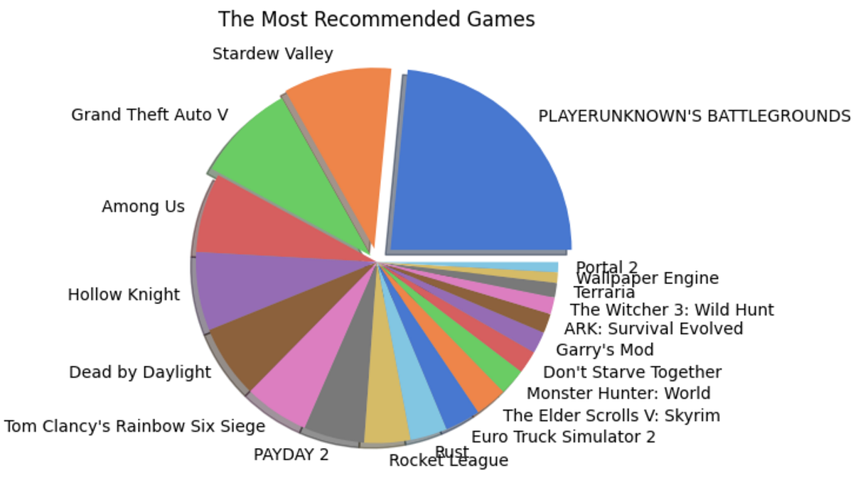
A complete guide to big data analysis using Apache Hadoop (HDFS) and PySpark library in Python on game reviews on the Steam gaming platform.With over 100 zettabytes (= 10¹²GB) of data produced every year around the world, the significance of handling big data is one of the most required skills today. Data Analysis, itself, could be defined as the ability to handle big data and derive insights from the never-ending and exponentially growing data. Apache Hadoop and Apache Spark are two of the basic tools that help us untangle the limitless possibilities hidden in large datasets. Apache Hadoop enables us to streamline data storage and distributed computing with its Distributed File System (HDFS) and the MapReduce-based parallel processing of data. Apache Spark is a big data analytics engine capable of EDA, SQL analytics, Streaming, Machine Learning, and Graph processing compatible with the major programming languages through its APIs. Both when combined form an exceptional environment for dealing with big data with the available computational resources — just a personal computer in most cases!Let us unfold the power of Big Data and Apache Hadoop with a simple analysis project implemented using Apache Spark in Python.To begin with, let's dive into the installation of Hadoop Distributed File System and Apache Spark on a MacOS. I am using a MacBook Air with macOS Sonoma with an M1 chip.Jump to the section —Installing Hadoop Distributed File SystemInstalling Apache SparkSteam Review Analysis using PySparkWhat next?1. Installing Hadoop Distributed File SystemThanks to Code With Arjun for the amazing article that helped me with the installation of Hadoop on my Mac. I seamlessly installed and ran Hadoop following his steps which I will show you here as well.a. Installing HomeBrewI use Homebrew for installing applications on my Mac for ease. It can be directly installed on the system with the below code —/bin/bash -c "$(curl -fsSL https://raw.githubusercontent.com/Homebrew/install/HEAD/install.sh)"Once it is installed, you can run the simple code below to verify the installation.brew --versionFigure 1: Image by AuthorHowever, you will likely encounter an error saying, command not found, this is because the homebrew will be installed in a different location (Figure 2) and it is not executable from the current directory. For it to function, we add a path environment variable for the brew, i.e., adding homebrew to the .bash_profile.Figure 2: Image by AuthorYou can avoid this step by using the full path to Homebrew in your commands, however, it might become a hustle at later stages, so not recommended!echo ‘eval “$(/opt/homebrew/bin/brew shellenv)”' >> /Users/rindhujajohnson/.bash_profileeval “$(/opt/homebrew/bin/brew shellenv)”Now, when you try, brew --version, it should show the Homebrew version correctly.b. Installing HadoopDisclaimer! Hadoop is a Java-based application and is supported by a Java Development Kit (JDK) version older than 11, preferably 8 or 11. Install JDK before continuing.Thanks to Code With Arjun again for this video on JDK installation on MacBook M1.https://medium.com/media/978a938e8d7a981d1b79b65db7884829/hrefNow, we install the Hadoop on our system using the brew command.brew install hadoopThis command should install Hadoop seamlessly. Similar to the steps followed while installing HomeBrew, we should edit the path environment variable for Java in the Hadoop folder. The environment variable settings for the installed version of Hadoop can be found in the Hadoop folder within HomeBrew. You can use which hadoop command to find the location of the Hadoop installation folder. Once you locate the folder, you can find the variable settings at the below location. The below command takes you to the required folder for editing the variable settings (Check the Hadoop version you installed to avoid errors).cd /opt/homebrew/Cellar/hadoop/3.3.6/libexec/etc/hadoopYou can view the files in this folder using the ls command. We will edit the hadoop-env.sh to enable the proper running of Hadoop on the system.Figure 3: Image by AuthorNow, we have to find the path variable for Java to edit the hadoop-ev.sh file using the following command./usr/libexec/java_homeFigure 4: Image by AuthorWe can open the hadoop-env.sh file in any text editor. I used VI editor, you can use any editor for the purpose. We can copy and paste the path — Library/Java/JavaVirtualMachines/adoptopenjdk-11.jdk/Contents/Home at the export JAVA_HOME = position.Figure 5: hadoop-env.sh file opened in VI Text EditorNext, we edit the four XML files in the Hadoop folder.core-site.xml<configuration> <property> <name>fs.defaultFS</name> <value>hdfs://localhost:9000</value> </property></configuration>hdfs-site.xml<configuration> <property> <name>dfs.replication</name> <value>1</value> </property></configuration>mapred-site.xml<configuration> <property> <name>mapreduce.framework.name</name> <value>yarn</value> </property> <property> <name>mapreduce.application.classpath</name> <value>$HADOOP_MAPRED_HOME/share/hadoop/mapreduce/*:$HADOOP_MAPRED_HOME/share/hadoop/mapreduce/lib/* </value> </property></configuration>yarn-site.xml<configuration> <property> <name>yarn.nodemanager.aux-services</name> <value>mapreduce_shuffle</value> </property> <property> <name>yarn.nodemanager.env-whitelist</name> <value>JAVA_HOME,HADOOP_COMMON_HOME,HADOOP_HDFS_HOME,HADOOP_CONF_DIR,CLASSPATH_PREPEND_DISTCACHE,HADOOP_YARN_HOME,HADOOP_MAPRED_HOME </value> </property></configuration>With this, we have successfully completed the installation and configuration of HDFS on the local. To make the data on Hadoop accessible with Remote login, we can go to Sharing in the General settings and enable Remote Login. You can edit the user access by clicking on the info icon.Figure 6: Enable Remote Access. Image by AuthorLet's run Hadoop!Execute the following commandshadoop namenode -format # starts the Hadoop environment% start-all.sh # Gathers all the nodes functioning to ensure that the installation was successful% jps Figure 7: Initiating Hadoop and viewing the nodes and resources running. Image by AuthorWe are all set! Now let's create a directory in HDFS and add the data will be working on. Let's quickly take a look at our data source and details.DataThe Steam Reviews Dataset 2021 (License: GPL 2) is a collection of reviews from about 21 million gamers covering over 300 different games in the year 2021. the data is extracted using Steam's API — Steamworks — using the Get List function.GET store.steampowered.com/appreviews/<appid>?json=1The dataset consists of 23 columns and 21.7 million rows with a size of 8.17 GB (that is big!). The data consists of reviews in different languages and a boolean column that tells if the player recommends the game to other players. We will be focusing on how to handle this big data locally using HDFS and analyze it using Apache Spark in Python using the PySpark library.c. Uploading Data into HDFSFirstly, we create a directory in the HDFS using the mkdir command. It will throw an error if we try to add a file directly to a non-existing folder.hadoop fs -mkdir /userhadoop fs - mkdir /user/steam_analysisNow, we will add the data file to the folder steam_analysis using the put command.hadoop fs -put /Users/rindhujajohnson/local_file_path/steam_reviews.csv /user/steam_analysisApache Hadoop also uses a user interface available at http://localhost:9870/.Figure 8: HDFS User Interface at localhost:9870. Image by AuthorWe can see the uploaded files as shown below.Figure 10: Navigating files in HDFS. Image by AuthorOnce the data interaction is over, we can use stop-all.sh command to stop all the Apache Hadoop daemons.Let us move to the next step — Installing Apache Spark2. Installing Apache SparkApache Hadoop takes care of data storage (HDFS) and parallel processing (MapReduce) of the data for faster execution. Apache Spark is a multi-language compatible analytical engine designed to deal with big data analysis. We will run the Apache Spark on Python in Jupyter IDE.After installing and running HDFS, the installation of Apache Spark for Python is a piece of cake. PySpark is the Python API for Apache Spark that can be installed using the pip method in the Jupyter Notebook. PySpark is the Spark Core API with its four components — Spark SQL, Spark ML Library, Spark Streaming, and GraphX. Moreover, we can access the Hadoop files through PySpark by initializing the installation with the required Hadoop version.# By default, the Hadoop version considered will be 3 here.PYSPARK_HADOOP_VERSION=3 pip install pysparkLet's get started with the Big Data Analytics!3. Steam Review Analysis using PySparkSteam is an online gaming platform that hosts over 30,000 games streaming across the world with over 100 million players. Besides gaming, the platform allows the players to provide reviews for the games they play, a great resource for the platform to improve customer experience and for the gaming companies to work on to keep the players on edge. We used this review data provided by the platform publicly available on Kaggle.3. a. Data Extraction from HDFSWe will use the PySpark library to access, clean, and analyze the data. To start, we connect the PySpark session to Hadoop using the local host address.from pyspark.sql import SparkSessionfrom pyspark.sql.functions import *# Initializing the Spark Sessionspark = SparkSession.builder.appName("SteamReviewAnalysis").master("yarn").getOrCreate()# Providing the url for accessing the HDFSdata = "hdfs://localhost:9000/user/steam_analysis/steam_reviews.csv"# Extracting the CSV data in the form of a Schemadata_csv = spark.read.csv(data, inferSchema = True, header = True)# Visualize the structure of the Schemadata_csv.printSchema()# Counting the number of rows in the datasetdata_csv.count() # 40,848,6593. b. Data Cleaning and Pre-ProcessingWe can start by taking a look at the dataset. Similar to the pandas.head() function in Pandas, PySpark has the SparkSession.show() function that gives a glimpse of the dataset.Before that, we will remove the reviews column in the dataset as we do not plan on performing any NLP on the dataset. Also, the reviews are in different languages making any sentiment analysis based on the review difficult.# Dropping the review column and saving the data into a new variabledata = data_csv.drop("review")# Displaying the datadata.show() Figure 11: The Structure of the SchemaWe have a huge dataset with us with 23 attributes with NULL values for different attributes which does not make sense to consider any imputation. Therefore, I have removed the records with NULL values. However, this is not a recommended approach. You can evaluate the importance of the available attributes and remove the irrelevant ones, then try imputing data points to the NULL values.# Drops all the records with NULL valuesdata = data.na.drop(how = "any")# Count the number of records in the remaining datasetdata.count() # 16,876,852We still have almost 17 million records in the dataset!Now, we focus on the variable names of the dataset as in Figure 11. We can see that the attributes have a few characters like dot(.) that are unacceptable as Python identifiers. Also, we change the data type of the date and time attributes. So we change these using the following code —from pyspark.sql.types import *from pyspark.sql.functions import from_unixtime# Changing the data type of each columns into appropriate typesdata = data.withColumn("app_id",data["app_id"].cast(IntegerType())). withColumn("author_steamid", data["author_steamid"].cast(LongType())). withColumn("recommended", data["recommended"].cast(BooleanType())). withColumn("steam_purchase", data["steam_purchase"].cast(BooleanType())). withColumn("author_num_games_owned", data["author_num_games_owned"].cast(IntegerType())). withColumn("author_num_reviews", data["author_num_reviews"].cast(IntegerType())). withColumn("author_playtime_forever", data["author_playtime_forever"].cast(FloatType())). withColumn("author_playtime_at_review", data["author_playtime_at_review"].cast(FloatType()))# Converting the time columns into timestamp data typedata = data.withColumn("timestamp_created", from_unixtime("timestamp_created").cast("timestamp")). withColumn("author_last_played", from_unixtime(data["author_last_played"]).cast(TimestampType())). withColumn("timestamp_updated", from_unixtime(data["timestamp_updated"]).cast(TimestampType()))Figure 12: A glimpse of the Steam review Analysis dataset. Image by AuthorThe dataset is clean and ready for analysis!3. c. Exploratory Data AnalysisThe dataset is rich in information with over 20 variables. We can analyze the data from different perspectives. Therefore, we will be splitting the data into different PySpark data frames and caching them to run the analysis faster.# Grouping the columns for each analysiscol_demo = ["app_id", "app_name", "review_id", "language", "author_steamid", "timestamp_created" ,"author_playtime_forever","recommended"]col_author = ["steam_purchase", 'author_steamid', "author_num_games_owned", "author_num_reviews", "author_playtime_forever", "author_playtime_at_review", "author_last_played","recommended"]col_time = [ "app_id", "app_name", "timestamp_created", "timestamp_updated", 'author_playtime_at_review', "recommended"]col_rev = [ "app_id", "app_name", "language", "recommended"]col_rec = ["app_id", "app_name", "recommended"]# Creating new pyspark data frames using the grouped columnsdata_demo = data.select(*col_demo)data_author = data.select(*col_author)data_time = data.select(*col_time)data_rev = data.select(*col_rev)data_rec = data.select(*col_rec)i. Games AnalysisIn this section, we will try to understand the review and recommendation patterns for different games. We will consider the number of reviews analogous to the popularity of the game and the number of True recommendations analogous to the gamer's preference for the game.Finding the Most Popular Games# the data frame is grouped by the game and the number of occurrences are countedapp_names = data_rec.groupBy("app_name").count()# the data frame is ordered depending on the count for the highest 20 gamesapp_names_count = app_names.orderBy(app_names["count"].desc()).limit(20)# a pandas data frame is created for plottingapp_counts = app_names_count.toPandas()# A pie chart is createdfig = plt.figure(figsize = (10,5))colors = sns.color_palette("muted")explode = (0.1,0.075,0.05,0,0,0,0,0,0,0,0,0,0,0,0,0,0,0,0,0)plt.pie(x = app_counts["count"], labels = app_counts["app_name"], colors = colors, explode = explode, shadow = True)plt.title("The Most Popular Games")plt.show()Finding the Most Recommended Games# Pick the 20 highest recommended games and convert it in to pandas data frametrue_counts = data_rec.filter(data_rec["recommended"] == "true").groupBy("app_name").count()recommended = true_counts.orderBy(true_counts["count"].desc()).limit(20)recommended_apps = recommended.toPandas()# Pick the games such that both they are in both the popular and highly recommended listtrue_apps = list(recommended_apps["app_name"])true_app_counts = data_rec.filter(data_rec["app_name"].isin(true_apps)).groupBy("app_name").count()true_app_counts = true_app_counts.orderBy(true_app_counts["count"].desc())true_app_counts = true_app_counts.toPandas()# Evaluate the percent of true recommendations for the top games and sort themtrue_perc = []for i in range(0,20,1): percent = (true_app_counts["count"][i]-recommended_apps["count"][i])/true_app_counts["count"][i]*100 true_perc.append(percent)recommended_apps["recommend_perc"] = true_percrecommended_apps = recommended_apps.sort_values(by = "recommend_perc", ascending = False)# Built a pie chart to visualizefig = plt.figure(figsize = (10,5))colors = sns.color_palette("muted")explode = (0.1,0.075,0.05,0,0,0,0,0,0,0,0,0,0,0,0,0,0,0,0,0)plt.pie(x = recommended_apps["recommend_perc"], labels = recommended_apps["app_name"], colors = colors, explode = explode, shadow = True)plt.title("The Most Recommended Games")plt.show()Figure 13: Shows the pie charts for popular and recommended games. Images by AuthorInsightsPlayer Unknown's Battlegrounds (PUBG) is the most popular and most recommended game of 2021.However, the second positions for the two categories are held by Grand Theft Auto V (GTA V) and Stardew Valley respectively. This shows that being popular does not mean all the players recommend the game to another player.The same pattern is observed with other games also. However, the number of reviews for a game significantly affects this trend.ii. Demographic AnalysisWe will find the demography, especially, the locality of the gamers using the data_demo data frame. This analysis will help us understand the popular languages used for review and languages used by reviewers of popular games. We can use this trend to determine the demographic influence and sentiments of the players to be used for recommending new games in the future.Finding Popular Review Languages# We standardize the language names in the language column, then group them,# Count by the groups and convert into pandas df after sorting them the countauthor_lang = data_demo.select(lower("language").alias("language")) .groupBy("language").count().orderBy(col("count").desc()). limit(20).toPandas()# Plotting a bar graphfig = plt.figure(figsize = (10,5))plt.bar(author_lang["language"], author_lang["count"])plt.xticks(rotation = 90)plt.xlabel("Popular Languages")plt.ylabel("Number of Reviews (in Millions)")plt.show()Finding Review Languages of Popular Games# We group the data frame based on the game and language and count each occurrencedata_demo_new = data_demo.select(lower("language"). alias("language"), "app_name")games_lang = data_demo_new.groupBy("app_name","language").count().orderBy(col("count").desc()).limit(100).toPandas()# Plot a stacked bar graph to visualizegrouped_games_lang = games_lang_df.pivot(index='app_name', columns='language', values='count')grouped_games_lang.plot(kind='bar', stacked=True, figsize=(12, 6))plt.title('Count of Different App Names and Languages')plt.xlabel('App Name')plt.ylabel('Count')plt.show()Figure 14: Language Popularity; Language Popularity among Popular games. Images by AuthorInsightsEnglish is the most popular language used by reviewers followed by Schinese and RussianSchinese is the most widely used language for the most popular game (PUBG), whereas, English is widely used for the second most popular game (GTA V) and almost all others!The popularity of a game seems to have roots in the area of origin. PUBG is a product of a South Korean gaming company and we observe that it has the Korean language among one of the highly used.Time, author, and review analyses are also performed on this data, however, do not give any actionable insights. Feel free to visit the GitHub repository for the full project documentation.3. d. Game Recommendation using Spark ML LibraryWe have reached the last stage of this project, where we will implement the Alternating Least Squares (ALS) machine-learning algorithm from the Spark ML Library. This model utilizes the collaborative filtering technique to recommend games based on player's behavior, i.e., the games they played before. This algorithm identifies the game selection pattern for players who play each available game on the Steam App.For the algorithm to work,We require three variables — the independent variable, target variable(s) — depending on the number of recommendations, here 5, and a rating variable.We encode the games and the authors to make the computation easier. We also convert the booleanrecommended column into a rating column with True = 5, and False = 1.Also, we will be recommending 5 new games for each played game and therefore we consider the data of the players who have played more than five for modeling the algorithm.Let's jump to the modeling and recommending part!new_pair_games = data_demo.filter(col("author_playtime_forever")>=5*mean_playtime)new_pair_games = new_pair_games.filter(new_pair_games["author_steamid"]>=76560000000000000).select("author_steamid","app_id", "app_name","recommended")# Convert author_steamid and app_id to indices, and use the recommended column for ratingauthor_indexer = StringIndexer(inputCol="author_steamid", outputCol="author_index").fit(new_pair_games)app_indexer = StringIndexer(inputCol="app_name", outputCol="app_index").fit(new_pair_games)new_pair_games = new_pair_games.withColumn("Rating", when(col("recommended") == True, 5).otherwise(1))# We apply the indexing to the data frame by invoking the reduce phase function transform()new_pair = author_indexer.transform(app_indexer.transform(new_pair_games))new_pair.show()# The reference chart for gamesgames = new_pair.select("app_index","app_name").distinct().orderBy("app_index")Figure 16: The game list with the corresponding index for reference. Image by AuthorImplementing ALS Algorithm# Create an ALS (Alternating Least Squares) modelals = ALS(maxIter=10, regParam=0.01, userCol="app_index", itemCol="author_index", ratingCol="Rating", coldStartStrategy="drop")# Fit the model to the datamodel = als.fit(new_pair)# Generate recommendations for all itemsapp_recommendations = model.recommendForAllItems(5) # Number of recommendations per item# Display the recommendationsapp_recommendations.show(truncate=False)Figure 17: The recommendation and rating generated for each author based on their gaming history. Image by AuthorWe can cross-match the indices from Figure 16 to find the games recommended for each player. Thus, we implemented a basic recommendation system using the Spark Core ML Library.3. e. ConclusionIn this project, we could successfully implement the following —Download and install the Hadoop ecosystem — HDFS and MapReduce — to store, access, and extract big data efficiently, and implement big data analytics much faster using a personal computer.Install the Apache Spark API for Python (PySpark) and integrate it with the Hadoop ecosystem, enabling us to carry out big data analytics and some machine-learning operations.The games and demographic analysis gave us some insights that can be used to improve the gaming experience and control the player churn. Keeping the players updated and informed about the trends in their peers should be a priority for the Steam platform. Suggestions like “most played”, “most played in your region”, “most recommended”, and “don't miss out on these new games” can keep the players active.The Steam Application can use the ALS recommendation system to recommend new games to existing players based on their profile and keep them engaged and afresh.4. What Next?Implement Natural Language Processing techniques in the review column, for different languages to extract the essence of the reviews and improve the gaming experience.Steam can report bugs in the games based on the reviews. Developing an AI algorithm that captures the review content, categorizes it, and sends it to appropriate personnel could do wonders for the platform.Comment what you think can be done more!5. ReferencesApache Hadoop. Apache Hadoop. Apache HadoopStatista. (2021). Volume of data/information created, captured, copied, and consumed worldwide from 2010 to 2020, with forecasts from 2021 to 2025 statistaDey, R. (2023). A Beginner's Guide to Big Data and Hadoop Distributed File System (HDFS). MediumCode with Arjun (2021). Install Hadoop on Mac OS (MacBook M1). MediumApache Spark. PySpark Installation. Apache SparkApache Spark. Collaborative Filtering with ALS). Apache SparkLet's Uncover it. (2023). PUBG. Let's Uncover ItYou can find the complete big data analysis project in my GitHub repository.Let's connect on LinkedIn and discuss more!If you found this article useful, clap, share, and comment!Apache Hadoop and Apache Spark for Big Data Analysis was originally published in Towards Data Science on Medium, where people are continuing the conversation by highlighting and responding to this story.
Apache Hadoop and Apache Spark for Big Data Analysis...
A complete guide to big data analysis using Apache Hadoop (HDFS) and PySpark library...
Source: Towards Data Science
Apple dévoile la puce M4 ! Bienvenu dans l'ère des iPhones dopés à l'IA

A l'occasion de l'évènement « Let Loose », Apple a lancé sa nouvelle puce M4. Cette dernière se focalise davantage … Cet article Apple dévoile la puce M4 ! Bienvenu dans l'ère des iPhones dopés à l'IA a été publié sur LEBIGDATA.FR.
Apple dévoile la puce M4 ! Bienvenu dans l'ère...
A l'occasion de l'évènement « Let Loose », Apple a lancé sa nouvelle puce M4....
Source: Le Big Data